Companion page: Chapter 5 Matlab resources — commands for trying out the material below on a machine.
Apart from \(Ax=b\), a second matrix problem keeps turning up in engineering. Given a square matrix \(A\), find the numbers \(\lambda\) and the nonzero vectors \(x\) with
When \(A\), \(\lambda\) and \(x\) are real, such an \(x\) is a vector that \(A\) does not turn: it only stretches it, shrinks it or reverses it, by the factor \(\lambda\). Chapter 4 was written with this problem in mind, and its Theorem 4.5 — a square matrix is singular exactly when its determinant is zero — is where this chapter starts.
1. Where eigenvalue problems come from
Take a one-dimensional cavity: two perfectly conducting walls at \(z=0\) and \(z=1\), with an electric field \(E(z,t)\) between them. (Position is called \(z\) in this section because \(x\) is reserved for the eigenvector.) The field obeys the wave equation and vanishes at the walls,
where \(c\) is the speed of light in the medium filling the cavity. Look for a field that oscillates at a single frequency \(\omega\), of the form \(E(z,t) = E_0(z)\,e^{j\omega t}\), where \(j = \sqrt{-1}\). Each time derivative brings down a factor \(j\omega\), so \(\partial^2E/\partial t^2 = -\omega^2E\), and the spatial profile \(E_0\) must satisfy
Now discretize exactly as Chapter 1 did for Poisson’s equation: \(n\) interior grid points \(z_k = kh\) with \(h = 1/(n+1)\), samples \(w_k = E_0(z_k)\), with \(w_0 = w_{n+1} = 0\) at the walls, and the centred second difference for the second derivative. Multiplying through by \(-h^2\), the equation at grid point \(k\) becomes
which in matrix form is
where \(w = (w_1,\ldots,w_n)^T\) and \(K\) is the \(n\times n\) matrix that Chapter 1 arrived at, with \(2\) on the diagonal and \(-1\) on either side of it (Chapter 4 calls it the second-difference matrix).
In Chapter 1 the right-hand side was a known charge density and the potential was the unknown. Here there is no right-hand side. Both \(w\) and \(\lambda\) are unknown, and \(w=0\) satisfies (5) for every \(\lambda\) while describing no field at all. The question is which values of \(\lambda\) allow a nonzero \(w\). Each such \(\lambda\) (for this \(K\) they all turn out to be positive) gives, through \(\lambda = (\omega h/c)^2\), a frequency \(\omega = (c/h)\sqrt{\lambda}\) at which the cavity can hold a standing field, and the corresponding \(w\) is the shape of that field at the grid points. They approximate some of the frequencies and field shapes that (3) allows (which has infinitely many), and only as well as the finite difference that produced (5) approximates the second derivative. In three dimensions the same steps turn \(\nabla^2\) into a larger matrix and lead to the same kind of problem.
The cavity is one example of many. A good number of engineering problems are eigenvalue problems in disguise, once they are written in matrix form:
-
the natural frequencies and mode shapes of a vibrating structure, such as a bridge, a building or a guitar string;
-
the resonant frequencies of a network of inductors and capacitors, and the modes that a waveguide or an optical fibre can carry;
-
the behaviour of a linear system \(du/dt = Au\): a solution of the form \(e^{\lambda t}x\) needs \(Ax = \lambda x\), and the eigenvalues \(\lambda\) decide whether it grows, decays or oscillates;
-
the long-run state of a Markov chain, such as the ranking of web pages by a search engine, which is an eigenvector with eigenvalue \(1\);
-
the directions along which a data set varies the most (principal component analysis), which are eigenvectors of its covariance matrix;
-
the energy levels of an atom, which are the eigenvalues in Schrödinger’s equation.
In each case the matrix is known, and the question is the one the cavity asked: which vectors does the matrix only scale, and by how much.
2. The eigenvalue problem
Let \(A\) be an \(n\times n\) matrix. A number \(\lambda\) is an eigenvalue of \(A\), and a vector \(x\) is an eigenvector of \(A\) belonging to \(\lambda\), if
A few remarks on this definition.
-
The problem makes sense only for square matrices: if \(A\) were \(m\times n\), then \(Ax\) would have \(m\) entries and \(\lambda x\) would have \(n\).
-
\(x = 0\) is excluded because \(A0 = \lambda 0\) for every \(\lambda\), which says nothing. \(\lambda = 0\) is allowed: an eigenvector for \(\lambda=0\) is simply a nonzero vector in the null space of \(A\).
-
An eigenvector is fixed only up to a nonzero scalar multiple. If \(Ax = \lambda x\) then \(A(cx) = \lambda(cx)\) for every \(c \neq 0\). So \((1,1)^T\) and \((3,3)^T\) are equally good eigenvectors, and so are \((1,0)^T\) and \((j,0)^T\), the second being \(j\) times the first.
-
Both \(\lambda\) and \(x\) are allowed to be complex, even when \(A\) is real; Section 3.4 shows a real \(2\times 2\) matrix whose eigenvalues are \(\pm j\). The results of earlier chapters used below — elimination and Theorem 1.9 from Chapter 1, Theorem 2.7 from Chapter 2, and Theorems 4.2 to 4.6 from Chapter 4 — were stated for real matrices, but their proofs use nothing beyond addition, subtraction, multiplication and division of the entries. So they hold unchanged for complex matrices (with the same assumption Chapter 4 made, that a function obeying its Rules 1 to 3 exists), and they are used that way from here on. In the same way, Chapter 2’s definitions of subspace, span, independence, basis and dimension are used with complex numbers allowed as the scalars in every combination.
To find the eigenvalues, rewrite \(Ax = \lambda x\) as \((A - \lambda I)x = 0\). By Theorem 1.9, a nonzero solution \(x\) exists exactly when \(A - \lambda I\) is not invertible, i.e. singular. By Theorem 4.5, \(A-\lambda I\) is singular exactly when
So \(\lambda\) is an eigenvalue of \(A\) if and only if it satisfies (6), and the eigenvectors belonging to it are the nonzero vectors of the null space \(N(A-\lambda I)\).
The left side of (6), as a function of \(\lambda\), is the characteristic polynomial of \(A\),
Theorem 5.1. Let \(A\) be an \(n\times n\) matrix. Then \(p_A(\lambda)\) is a polynomial in \(\lambda\) of degree \(n\), and its \(\lambda^n\) term is \((-1)^n\lambda^n\).
This is stated here without proof. For \(n=2\) it can be checked directly (Section 4). For general \(n\) it needs a formula for the determinant in terms of the entries, such as the cofactor expansion of GS §4.3.
To go further we need one fact from algebra, quoted here without proof. The fundamental theorem of algebra says that a polynomial of degree \(n \geq 1\) with complex coefficients has exactly \(n\) complex roots when each root is counted as often as it is repeated, and that the polynomial equals its leading coefficient times the product of the factors \((\lambda - \text{root})\) over these roots. The roots, with their repetitions, are determined by the polynomial, uniquely apart from the order in which they are listed. Applied to \(p_A\), whose leading coefficient is \((-1)^n\) by Theorem 5.1, this says that there are complex numbers \(\lambda_1,\ldots,\lambda_n\), not necessarily distinct and unique apart from their order, with
(Each factor \(\lambda_i - \lambda\) contributes a \(-\lambda\), which is where the \((-1)^n\) goes.) The \(\lambda_i\) are the roots of \(p_A\), so they are the eigenvalues of \(A\), and the list \(\lambda_1,\ldots,\lambda_n\) counts each eigenvalue as many times as its factor appears. In this sense an \(n\times n\) matrix has \(n\) eigenvalues, possibly complex and possibly repeated.
The eigenvalue problem is therefore solved in two steps: first find the eigenvalues as the roots of \(p_A(\lambda) = 0\), and then, for each eigenvalue \(\lambda\), find the eigenvectors by solving \((A - \lambda I)x = 0\). The second step is elimination, as in Chapter 2. The first step is the hard one. A polynomial of degree \(n \geq 5\) has no general formula for its roots built from its coefficients by arithmetic and the extraction of roots (GS §5.1 mentions this). In practice the eigenvalues of a large matrix are computed by iterative numerical methods, which do not go through \(p_A\) at all.
3. Examples
3.1. A \(2\times 2\) matrix
Take
Then
so the eigenvalues are \(\lambda_1 = -1\) and \(\lambda_2 = 2\). For each, solve \((A-\lambda I)x = 0\):
So \(u = (1,1)^T\) is an eigenvector for \(-1\) and \(v = (5,2)^T\) is one for \(2\). Check: \(Au = (4-5,\,2-3)^T = (-1,-1)^T = -u\) and \(Av = (20-10,\,10-6)^T = (10,4)^T = 2v\). In both cases the two rows of \(A - \lambda I\) are multiples of each other, as they must be: the matrix is singular, so the two equations carry only one condition between them.
3.2. Triangular matrices
Theorem 5.2. If \(A\) is triangular, its eigenvalues \(\lambda_1,\ldots,\lambda_n\) in (7) are its diagonal entries \(a_{11},\ldots,a_{nn}\).
Proof
\(A - \lambda I\) is triangular too, with diagonal entries \(a_{ii} - \lambda\). By Theorem 4.4 its determinant is the product of those entries,
which is already of the form (7). Since the list of eigenvalues in (7) is unique apart from its order, the eigenvalues, counted with repetition, are \(a_{11},\ldots,a_{nn}\).
So for a triangular matrix the eigenvalues can be read off the diagonal. Elimination changes the eigenvalues, though: the \(2\times 2\) example above reduces to an upper triangular \(U\) with the pivots \(4\) and \(-1/2\) on its diagonal (subtracting \(\tfrac12\) times row 1 from row 2 leaves \(-3 - \tfrac12(-5) = -\tfrac12\) in the \((2,2)\) place), while its eigenvalues are \(2\) and \(-1\).
3.3. Projections
Take the projection onto the line through \(a = (1,1)^T\) from Chapter 3,
The donkey’s way is to grind through the algorithm:
so the eigenvalues are \(0\) and \(1\). For \(\lambda = 0\), \(Px = 0\) gives \(x_1 + x_2 = 0\) and the eigenvector \((1,-1)^T\). For \(\lambda = 1\), \((P - I)x = 0\) has rows \((-\tfrac12, \tfrac12)\) and \((\tfrac12,-\tfrac12)\), giving \(x_1 = x_2\) and the eigenvector \((1,1)^T\).
The owl’s way needs no algebra at all. \(P\) sends every vector to its shadow on the line through \(a\). A vector on the line is its own shadow, so \(Pa = a\) and \(a\) is an eigenvector with eigenvalue \(1\). A vector perpendicular to the line has zero shadow, so it is an eigenvector with eigenvalue \(0\). Any other vector, like \(v_2\) in Figure 1, has a shadow \(Pv_2\) that lies along \(a\), so \(Pv_2\) is not a multiple of \(v_2\), and \(v_2\) is not an eigenvector.
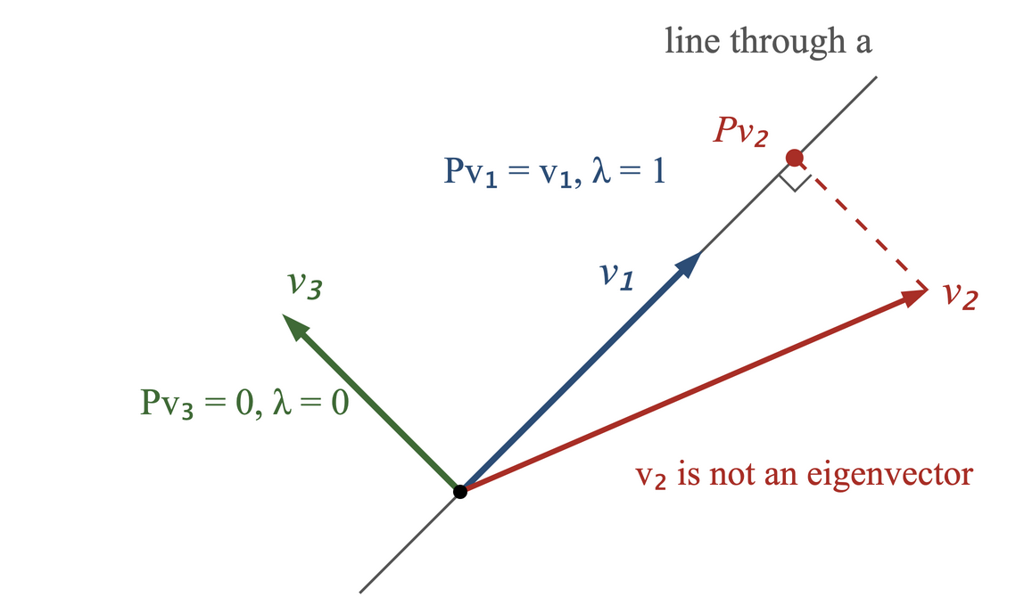
Whatever the projection, its eigenvalues can only be \(0\) or \(1\).
Theorem 5.3. If \(P\) is an \(n\times n\) matrix with \(P^2 = P\), then every eigenvalue of \(P\) is \(0\) or \(1\).
Proof
Let \(Px = \lambda x\) with \(x \neq 0\). Applying \(P\) once more, \(P^2x = \lambda Px = \lambda^2 x\). But \(P^2 = P\), so \(P^2x = Px = \lambda x\). Hence \(\lambda^2 x = \lambda x\), i.e. \((\lambda^2 - \lambda)x = 0\), and since \(x \neq 0\) this forces \(\lambda^2 - \lambda = 0\), i.e. \(\lambda = 0\) or \(\lambda = 1\).
The theorem says only that \(0\) and \(1\) are the only candidates. Both need not occur: \(P = I\) has only the eigenvalue \(1\), and \(P = 0\) only the eigenvalue \(0\). Combined with (7), it says that the characteristic polynomial of an \(n\times n\) matrix with \(P^2 = P\) is \(p_P(\lambda) = (-\lambda)^a(1-\lambda)^b\) with \(a + b = n\): the eigenvalue \(0\) repeated \(a\) times and \(1\) repeated \(b\) times.
It covers every projection matrix of Chapter 3, and the owl’s picture carries over as well. For \(P = M(M^TM)^{-1}M^T\), the projection onto the column space of a matrix \(M\) with independent columns, \(P^2 = P\) by Theorem 3.13. A vector \(b = My\) in \(C(M)\) satisfies \(Pb = M(M^TM)^{-1}(M^TM)y = My = b\), so every nonzero vector of \(C(M)\) is an eigenvector with eigenvalue \(1\). A vector \(b\) in \(N(M^T)\) has \(M^Tb = 0\) and so \(Pb = 0\), so every nonzero vector of \(N(M^T)\) is an eigenvector with eigenvalue \(0\).
The projection need not be onto a line. The \(4\times 4\) matrix
satisfies \(P^2 = P\): it projects onto the plane spanned by \(e_1\) and \(e_4\). It is diagonal, so by Theorem 5.2 its eigenvalues are \(1, 0, 0, 1\). The vectors \(e_1\) and \(e_4\) are eigenvectors for \(1\), and \(e_2\) and \(e_3\) are eigenvectors for \(0\). So an eigenvalue can be repeated, and a repeated eigenvalue can have more than one independent eigenvector. Counting these two things is the subject of Section 5.
3.4. A rotation
The matrix
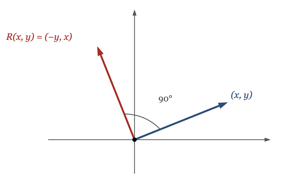
rotates every vector of the plane through \(90^\circ\) (Figure 2). No nonzero real vector comes out parallel to itself, so the owl sees at once that \(R\) has no real eigenvector.
The algebra still produces eigenvalues:
For \(\lambda = j\), the first row of \((R - jI)x = 0\) reads \(-jx_1 - x_2 = 0\), so \(x_2 = -jx_1\); taking \(x_1 = j\) gives the eigenvector \((j, 1)^T\). For \(\lambda = -j\), the first row of \((R + jI)x = 0\) reads \(jx_1 - x_2 = 0\), so \(x_2 = jx_1\); taking \(x_1 = j\) gives \((j,-1)^T\). Check the first: \(R(j,1)^T = (-1, j)^T\), and \(j(j,1)^T = (j^2, j)^T = (-1,j)^T\).
So a real matrix can have complex eigenvalues and complex eigenvectors. The eigenvectors live in \(\mathbb{C}^2\), which has four real dimensions, and that is why no picture drawn in the real plane shows them.
4. Trace and determinant
For a general \(2\times 2\) matrix,
This confirms Theorem 5.1 for \(n = 2\), and the quadratic formula gives the two eigenvalues as
On the other hand, by (7),
Two polynomials that agree for every \(\lambda\) have the same coefficients, so comparing with (8),
The sum of the diagonal entries of a square matrix is its trace, \(\operatorname{tr}A = a_{11} + a_{22} + \cdots + a_{nn}\). So for \(2\times 2\) matrices the eigenvalues add up to the trace and multiply to the determinant. Both statements hold for every \(n\).
Theorem 5.4. Let \(A\) be an \(n\times n\) matrix with eigenvalues \(\lambda_1,\ldots,\lambda_n\), counted with repetition as in (7). Then \(\lambda_1\lambda_2\cdots\lambda_n = \det A\).
Proof
Put \(\lambda = 0\) in (7). The left side is \(p_A(0) = \det(A - 0\cdot I) = \det A\), and the right side is \(\lambda_1\lambda_2\cdots\lambda_n\).
Theorem 5.5. Let \(A\) be an \(n\times n\) matrix with eigenvalues \(\lambda_1,\ldots,\lambda_n\), counted with repetition as in (7). Then \(\lambda_1 + \lambda_2 + \cdots + \lambda_n = \operatorname{tr}A\).
This was proved above for \(n = 2\) and is stated here without proof for general \(n\). A proof compares the coefficients of \(\lambda^{n-1}\) on the two sides of (7), and like Theorem 5.1 it needs a formula for the determinant in terms of the entries; GS §5.1 (Exercise 9) outlines one.
Both give quick checks on a computed set of eigenvalues. For the \(2\times 2\) example of Section 3.1, \(2 + (-1) = 1 = 4 + (-3)\) and \((2)(-1) = -2 = (4)(-3) - (-5)(2)\). For the projection \(P\) onto the line, \(0 + 1 = \tfrac12 + \tfrac12\) and \((0)(1) = 0 = \det P\). For the rotation, \(j + (-j) = 0 = \operatorname{tr}R\) and \((j)(-j) = -j^2 = 1 = (0)(0) - (-1)(1)\).
Theorem 5.4 also says that \(A\) is singular exactly when \(0\) is one of its eigenvalues. That agrees with the definition: \(\lambda = 0\) is an eigenvalue exactly when \(Ax = 0\) has a nonzero solution.
5. Algebraic and geometric multiplicity
Suppose \(A\) has \(d\) distinct eigenvalues. In this section the labels \(\lambda_1,\ldots,\lambda_d\) name these distinct values, each once, rather than the list with repetition used in (7) and in Theorems 5.4 and 5.5. Collecting the equal factors in (7),
The exponent \(\mu_A(\lambda_i)\) — the number of times \(\lambda_i\) is repeated in the list of eigenvalues — is the algebraic multiplicity of \(\lambda_i\). It is well defined because the list \(\lambda_1,\ldots,\lambda_n\) in (7) is unique apart from its order, and since the degrees on the two sides of (9) must agree,
The eigenvectors belonging to \(\lambda_i\) are the nonzero vectors of \(N(A-\lambda_i I)\). Being a null space, this is a subspace of \(\mathbb{C}^n\); it is called the eigenspace of \(\lambda_i\). Its dimension is the geometric multiplicity of \(\lambda_i\),
the second form by Theorem 2.7. In words, \(\gamma_A(\lambda_i)\) is the largest number of independent eigenvectors that \(\lambda_i\) has. It is at least \(1\): \(\lambda_i\) is an eigenvalue, so \(A - \lambda_iI\) is singular and its null space contains a nonzero vector. The two multiplicities count different things — repeated roots of a polynomial on one side, independent directions on the other — and the examples show that they need not agree.
-
\(A = I\), of size \(n\). Here \(p_I(\lambda) = (1-\lambda)^n\), so \(\lambda = 1\) is the only eigenvalue and \(\mu_I(1) = n\). And \(I - 1\cdot I\) is the zero matrix, whose null space is all of \(\mathbb{C}^n\), so \(\gamma_I(1) = n\). Every nonzero vector is an eigenvector.
-
\(A = \operatorname{diag}(1, 0, \ldots, 0)\), of size \(n \geq 2\). By Theorem 5.2 the eigenvalues are \(1\) once and \(0\) repeated \(n-1\) times, so \(\mu_A(1) = 1\) and \(\mu_A(0) = n-1\). The matrix \(A - 0\cdot I = A\) has rank \(1\), so \(\gamma_A(0) = n-1\), and \(A - I = \operatorname{diag}(0,-1,\ldots,-1)\) has rank \(n-1\), so \(\gamma_A(1) = 1\). The two multiplicities agree for both eigenvalues. (The \(4\times 4\) projection of Section 3.3 is the same kind of example.)
-
\(A = \begin{bmatrix} 0 & 1 \\ 0 & 0\end{bmatrix}\). It is triangular, so \(p_A(\lambda) = \lambda^2\) and \(\mu_A(0) = 2\). But \(A - 0\cdot I = A\) has rank \(1\), so \(\gamma_A(0) = 2 - 1 = 1\): the equation \(Ax = 0\) says \(x_2 = 0\), and every eigenvector is a multiple of \((1,0)^T\). The eigenvalue is repeated, but there is only one eigenvector direction.
The last example has \(\gamma < \mu\). The opposite never happens, and the rest of this section proves it. Two facts about determinants come first.
Lemma 5.6. Let \(M\) be a square matrix in the block form
where \(B\) and \(D\) are square (of any sizes) and the zero block sits below \(B\). Then \(\det M = \det B\,\det D\).
Proof
The plan is to bring \(M\) to upper triangular form by eliminating inside the two diagonal blocks separately, while keeping count of the row exchanges.
Let \(B\) be \(k\times k\). First run elimination, with row exchanges as needed, on the first \(k\) rows of \(M\), using only those rows. On the columns of \(B\) this is exactly elimination on \(B\), and it ends with an upper triangular \(B'\) (Chapter 1); the columns of \(C\) are carried along and become some \(C'\). The last rows of \(M\) are not touched.
Next run elimination on the last rows of \(M\), again using only those rows. Each of these rows is zero in the first \(k\) columns, so subtracting multiples of them from one another, or exchanging them, keeps those columns zero. On the columns of \(D\) this is exactly elimination on \(D\), and it ends with an upper triangular \(D'\). The result is
which is upper triangular, with the diagonal entries of \(B'\) followed by those of \(D'\).
Subtracting a multiple of one row from another changes no determinant (Theorem 4.2), and each row exchange reverses the sign (Rule 2). If \(r_1\) exchanges were made in the first stage and \(r_2\) in the second, then
By Theorem 4.4, \(\det M'\) is the product of its diagonal entries, which is the product of the diagonal entries of \(B'\) times that of \(D'\), i.e. \(\det M' = \det B'\,\det D'\). Putting these together,
The zero block below \(B\) is what makes \(M'\) triangular: the second stage starts with those columns zero in the last rows and keeps them zero.
Lemma 5.7. Let \(A\) and \(S\) be \(n\times n\), with \(S\) invertible. Then \(S^{-1}AS\) has the same characteristic polynomial as \(A\), and so the same eigenvalues with the same algebraic multiplicities.
Proof
Write \(\lambda I = \lambda S^{-1}S\), so that
By the product rule (Theorem 4.6) and \(\det(S^{-1}) = 1/\det S\) (equation (6) of Chapter 4),
This holds for every \(\lambda\), so \(p_{S^{-1}AS}\) and \(p_A\) are the same polynomial. They have the same factorization (9), which is the second claim.
Theorem 5.8. Let \(A\) be an \(n\times n\) matrix and \(\lambda_0\) an eigenvalue of \(A\). Then \(\gamma_A(\lambda_0) \leq \mu_A(\lambda_0)\).
Proof
The strategy is to build a basis of \(\mathbb{C}^n\) that begins with a full set of independent eigenvectors for \(\lambda_0\). Written in that basis, \(A\) becomes block triangular with \(\lambda_0 I\) in the top left corner, and its characteristic polynomial then visibly contains the factor \((\lambda_0-\lambda)\) repeated.
Since \(\lambda_0\) and its eigenvectors may be complex, we work in \(\mathbb{C}^n\) with the inner product \(x^Hy\), the complex form of \(x^Ty\) (Chapter 3 used \(x^Hx\) for lengths in \(\mathbb{C}^n\)); two vectors are orthogonal when \(x^Hy = 0\). Gram—Schmidt (Theorem 3.18) was proved in \(\mathbb{R}^n\) with \(x^Ty\); its proof, and Theorem 3.4 and Corollary 2.5 which it cites, go through unchanged with \(x^Hy\) in place of \(x^Ty\), the coefficient of \(q_i\) in step \(k\) becoming \(q_i^Ha_k\). When \(A\) and \(\lambda_0\) are real, the eigenvectors can be taken real (elimination on a real matrix never leaves the reals), every \({}^H\) below can be read as \({}^T\), and the proof is the one given in class.
Step 1: independent eigenvectors. Let \(r = \gamma_A(\lambda_0)\) and let \(v_1,\ldots,v_r\) be a basis of the eigenspace \(N(A - \lambda_0I)\).
Step 2: make them orthonormal. Apply Gram—Schmidt to \(v_1,\ldots,v_r\) to get orthonormal \(x_1,\ldots,x_r\). By Theorem 3.18 these span the same space as the \(v_k\), so each \(x_i\) is a combination \(\sum_k \alpha_k v_k\), and
Each \(x_i\) has length \(1\), so it is nonzero: the \(x_i\) are still eigenvectors for \(\lambda_0\).
Step 3: complete them to an orthonormal basis. Let \(X\) be the \(n\times r\) matrix whose columns are \(x_1,\ldots,x_r\). Orthonormality of the columns says \(X^HX = I_r\). A vector \(y\) is orthogonal to every \(x_i\) exactly when \(X^Hy = 0\), i.e. when \(y \in N(X^H)\). The \(r\) rows of \(X^H\) are independent: if \(wX^H = 0\) for a row vector \(w\), then \(w = wX^HX = 0\). So \(X^H\) has rank \(r\) (by Theorem 2.7, the rank is the dimension of the row space), and by the same theorem its null space has dimension \(n-r\). If \(r < n\), apply Gram—Schmidt to a basis of \(N(X^H)\) to get orthonormal \(y_1,\ldots,y_{n-r}\); being combinations of vectors of \(N(X^H)\), they lie in it, so \(x_i^Hy_k = 0\) (and hence \(y_k^Hx_i = 0\)) for all \(i\) and \(k\). Put all the vectors in the columns of
which is just \(S = X\) when \(r = n\). The columns of \(S\) are orthonormal — the \(x_i\) among themselves, the \(y_k\) among themselves, and each \(x_i\) against each \(y_k\) — which says \(S^HS = I\). So \(Sz = 0\) implies \(z = S^HSz = 0\), \(S\) is invertible by Theorem 1.9, and multiplying \(S^HS = I\) on the right by \(S^{-1}\) gives \(S^{-1} = S^H\).
Step 4: the block form. Write \(s_i\) for the \(i\)-th column of \(S\). Since \(S^{-1} = S^H\), the \((i,k)\) entry of \(S^{-1}AS\) is \(s_i^HAs_k\). For \(k \leq r\), \(As_k = Ax_k = \lambda_0 x_k\), so this entry is \(\lambda_0\,s_i^Hx_k\), which is \(\lambda_0\) when \(i = k\) and \(0\) otherwise, by orthonormality. If \(r = n\) this already gives \(S^{-1}AS = \lambda_0 I_n\), so \(p_A(\lambda) = (\lambda_0-\lambda)^n\) by Lemma 5.7 and Theorem 4.4, and, as in the proof of Theorem 5.2, \(\mu_A(\lambda_0) = n = r\), which proves the theorem in that case. In particular, when \(r < n\), in the first \(r\) columns every entry of rows \(r+1\) to \(n\) is \(y_i^H(\lambda_0x_k) = \lambda_0\, y_i^Hx_k = 0\), so
with \(C\) of size \(r\times(n-r)\) and \(D\) of size \((n-r)\times(n-r)\). Their entries do not matter.
Step 5: the characteristic polynomial. Subtracting \(\lambda I\) from (10) changes only the diagonal blocks:
By Lemma 5.6, and Theorem 4.4 for the diagonal block,
The left side is \(p_A(\lambda)\), by Lemma 5.7. On the right, \(\det(D - \lambda I_{n-r}) = p_D(\lambda)\) is the characteristic polynomial of the \((n-r)\times(n-r)\) matrix \(D\), which by Theorem 5.1 and the fundamental theorem of algebra factors as \((\nu_1 - \lambda)\cdots(\nu_{n-r}-\lambda)\), with \(\nu_1,\ldots,\nu_{n-r}\) the eigenvalues of \(D\). So
Step 6: conclusion. This displays \(p_A\) as \((-1)^n\) times the product of the \(n\) factors \((\lambda - \text{root})\) for the list \(\lambda_0\) (repeated \(r\) times), \(\nu_1,\ldots,\nu_{n-r}\). By the uniqueness in the fundamental theorem of algebra, that list is the list \(\lambda_1,\ldots,\lambda_n\) of (7), apart from order. In it \(\lambda_0\) appears at least \(r\) times: exactly \(r\) times if no \(\nu_k\) equals \(\lambda_0\), and more often if some do. Hence \(\mu_A(\lambda_0) \geq r = \gamma_A(\lambda_0)\).
Collecting the counts of this section:
Corollary 5.9. Let \(A\) be an \(n\times n\) matrix with distinct eigenvalues \(\lambda_1,\ldots,\lambda_d\). Then \(1 \leq \gamma_A(\lambda_i) \leq \mu_A(\lambda_i) \leq n\) for each \(i\), and
Proof
\(\gamma_A(\lambda_i) \geq 1\) was shown when \(\gamma\) was defined, and \(\gamma_A(\lambda_i) \leq \mu_A(\lambda_i)\) is Theorem 5.8. The algebraic multiplicities are positive integers adding up to \(n\), which gives both \(\mu_A(\lambda_i) \leq n\) and the sum. Adding \(\gamma_A(\lambda_i) \leq \mu_A(\lambda_i)\) over \(i\) gives \(\sum_i\gamma_A(\lambda_i) \leq n\); adding \(\gamma_A(\lambda_i) \geq 1\) over \(i\) gives \(\sum_i\gamma_A(\lambda_i) \geq d\); and \(d \geq 1\) because \(p_A\) has at least one root.
For the three examples above: \(I\) has \(\sum_i\gamma_A(\lambda_i) = n\), the maximum; so does \(\operatorname{diag}(1,0,\ldots,0)\), with \(1 + (n-1) = n\); and \(\begin{bmatrix} 0&1\\0&0\end{bmatrix}\) has \(\sum_i\gamma_A(\lambda_i) = 1 < 2\).
6. Diagonalization
Suppose the \(n\times n\) matrix \(A\) has \(n\) independent eigenvectors \(x_1,\ldots,x_n\), with \(Ax_i = \lambda_i x_i\). (Here the \(\lambda_i\) are indexed from 1 to \(n\), one per eigenvector, and need not be distinct.) Put the eigenvectors in the columns of a matrix \(S\). Then \(A\) acts on each column separately, and by the column picture
where \(\Lambda = \operatorname{diag}(\lambda_1,\ldots,\lambda_n)\). The columns of \(S\) are independent, so \(Sz = \sum_i z_ix_i = 0\) forces \(z = 0\), and \(S\) is invertible by Theorem 1.9. Multiplying (11) by \(S^{-1}\), on the right or on the left,
A square matrix \(A\) is diagonalizable if there is an invertible \(S\) with \(S^{-1}AS\) diagonal, and \(S^{-1}AS = \Lambda\) is called the diagonalization of \(A\). The argument also runs backwards: if \(S^{-1}AS = \Lambda\) is diagonal, then \(AS = S\Lambda\), which read column by column says that each column of \(S\) is an eigenvector of \(A\) with eigenvalue the corresponding diagonal entry of \(\Lambda\); and the columns of an invertible \(S\) are nonzero and independent. So \(A\) is diagonalizable exactly when it has \(n\) independent eigenvectors.
By Lemma 5.7 and Theorem 5.2, the diagonal of \(\Lambda\) then lists the eigenvalues of \(A\), each repeated as often as its algebraic multiplicity. The matrix \(S\) is not unique: each column can be scaled by any nonzero number, the columns can be reordered (with the diagonal of \(\Lambda\) reordered to match), and for a repeated eigenvalue any basis of its eigenspace will do (Theorem 5.12 below shows why).
When does \(A\) have \(n\) independent eigenvectors? Eigenvectors that belong to different eigenvalues are never a problem.
Theorem 5.10. Let \(x_1,\ldots,x_k\) be eigenvectors of a square matrix \(A\), belonging to eigenvalues \(\lambda_1,\ldots,\lambda_k\) that are all different. Then \(x_1,\ldots,x_k\) are linearly independent.
Proof
The idea, for two vectors, is this. Suppose \(c_1x_1 + c_2x_2 = 0\). Applying \(A\) gives \(c_1\lambda_1x_1 + c_2\lambda_2x_2 = 0\). Subtracting \(\lambda_1\) times the first equation from the second removes \(x_1\) and leaves \(c_2(\lambda_2-\lambda_1)x_2 = 0\). Since \(\lambda_2 \neq \lambda_1\) and \(x_2 \neq 0\), \(c_2 = 0\), and then \(c_1x_1 = 0\) gives \(c_1 = 0\).
For \(k\) vectors the same step removes one vector at a time, so we argue by induction on \(k\). For \(k=1\), a single eigenvector is nonzero and so independent. Assume the result for \(k-1\) eigenvectors, and suppose
Applying \(A\) gives \(c_1\lambda_1x_1 + \cdots + c_k\lambda_kx_k = 0\). Subtracting \(\lambda_k\) times the first equation from this one removes \(x_k\):
By the induction hypothesis \(x_1,\ldots,x_{k-1}\) are independent, so every coefficient \(c_i(\lambda_i - \lambda_k)\) is zero; and since \(\lambda_i \neq \lambda_k\), every \(c_i = 0\) for \(i \leq k-1\). What is left is \(c_kx_k = 0\), and \(x_k \neq 0\) gives \(c_k = 0\). So all the coefficients are zero, which is what independence means.
Corollary 5.11. If an \(n\times n\) matrix has \(n\) distinct eigenvalues, it is diagonalizable.
Proof
Take one eigenvector for each of the \(n\) eigenvalues. By Theorem 5.10 these \(n\) eigenvectors are independent, so \(A\) is diagonalizable.
For example, the rotation \(R\) of Section 3.4 has the two distinct eigenvalues \(j\) and \(-j\), so it is diagonalizable — with a complex \(S\). With the eigenvectors found there, \(S\) has columns \((j,1)^T\) and \((j,-1)^T\), and \(R = S\operatorname{diag}(j,-j)S^{-1}\). No real \(S\) can do this, since \(R\) has no real eigenvector.
Distinct eigenvalues are enough but not necessary: \(I\) has the single eigenvalue \(1\), repeated \(n\) times, and is already diagonal. With repeated eigenvalues the question is whether each eigenvalue has as many independent eigenvectors as it has repetitions.
Theorem 5.12. An \(n\times n\) matrix \(A\) is diagonalizable if and only if \(\gamma_A(\lambda_i) = \mu_A(\lambda_i)\) for every eigenvalue \(\lambda_i\).
Proof
Let \(\lambda_1,\ldots,\lambda_d\) be the distinct eigenvalues.
If. For each \(\lambda_i\) take a basis of its eigenspace \(N(A-\lambda_iI)\), of \(\gamma_A(\lambda_i)\) vectors, and put all these bases together. We show that the combined list is independent. Suppose a combination of all the vectors in the list is zero, and group its terms by eigenvalue: \(w_1 + w_2 + \cdots + w_d = 0\), where \(w_i\) is the part coming from the basis of the eigenspace of \(\lambda_i\). Each \(w_i\) lies in that eigenspace, so each nonzero \(w_i\) is an eigenvector for \(\lambda_i\). If some of the \(w_i\) were nonzero, the equation would say that eigenvectors for different eigenvalues add up to zero, which Theorem 5.10 rules out. So every \(w_i = 0\), and since each \(w_i\) is a combination of independent vectors, all its coefficients are zero. The combined list is therefore independent, and it has \(\sum_i\gamma_A(\lambda_i) = \sum_i\mu_A(\lambda_i) = n\) vectors (Corollary 5.9). So \(A\) has \(n\) independent eigenvectors and is diagonalizable.
Only if. Let \(A = S\Lambda S^{-1}\). The diagonal of \(\Lambda\) lists the eigenvalues with repetition, so exactly \(\mu_A(\lambda_i)\) columns of \(S\) are eigenvectors for \(\lambda_i\). They are independent and lie in \(N(A - \lambda_iI)\), and an independent set is never larger than the dimension of the space it lies in (Chapter 2, in the proof of Theorem 2.4), so \(\gamma_A(\lambda_i) \geq \mu_A(\lambda_i)\). With Theorem 5.8, the two are equal.
The matrix \(\begin{bmatrix} 0&1\\0&0\end{bmatrix}\) of Section 5 is the standard example of a matrix that cannot be diagonalized. Its eigenvalue \(0\) is repeated twice, but every eigenvector is a multiple of \((1,0)^T\), so no \(S\) with two independent eigenvector columns exists: \(\gamma_A(0) = 1 < 2 = \mu_A(0)\).
7. Powers and the inverse
The first use of (12) is to compute powers. The inner \(S^{-1}S\) pairs cancel:
with \(k\) factors, so that
Writing \(A = S\Lambda S^{-1}\) in this way is called the eigendecomposition of \(A\). Raising \(A\) to the power \(k\) by straightforward multiplication costs \(k-1\) matrix products; raising \(\Lambda\) to the power \(k\) only means raising \(n\) numbers to the power \(k\). By Lemma 5.7 and Theorem 5.2 applied to (13), the eigenvalues of \(A^k\) are the \(\lambda_i^k\). Every eigenvector of \(A\) with eigenvalue \(\lambda\) is an eigenvector of \(A^k\) with eigenvalue \(\lambda^k\), and this part needs no diagonalizability: if \(Ax = \lambda x\) then \(A^2x = \lambda Ax = \lambda^2x\), and so on. The converse fails: \(A^k\) can have eigenvectors that \(A\) does not. The rotation of Section 3.4 has \(R^2 = -I\), for which every nonzero vector is an eigenvector, while \(R\) has no real eigenvector.
The inverse works the same way. By Theorem 5.4, \(A\) is invertible exactly when none of its eigenvalues is zero, and then
as multiplying out \((S\Lambda S^{-1})(S\Lambda^{-1}S^{-1}) = I\) confirms. So the eigenvalues of \(A^{-1}\) are the reciprocals of those of \(A\), with the same eigenvectors. Again this holds whether or not \(A\) is diagonalizable: from \(Ax = \lambda x\) with \(\lambda \neq 0\), multiplying by \(A^{-1}\) gives \(x = \lambda A^{-1}x\), i.e. \(A^{-1}x = \tfrac{1}{\lambda}x\).
8. Products of matrices
Suppose \(Ax = \lambda x\) and \(By = \mu y\). Is \(\lambda\mu\) an eigenvalue of \(AB\)? Try it: \(ABy = A(\mu y) = \mu Ay\), and \(Ay\) is not a multiple of \(y\) unless \(y\) happens to be an eigenvector of \(A\) as well. Starting from the other side, \(BAx = \lambda Bx\) has the same problem. So nothing forces \(\lambda\mu\) to be an eigenvalue of \(AB\), and in general it is not. For example, \(A = \begin{bmatrix} 0&1\\0&0\end{bmatrix}\) and \(B = \begin{bmatrix} 0&0\\1&0\end{bmatrix}\) each have only the eigenvalue \(0\), but \(AB = \begin{bmatrix} 1&0\\0&0\end{bmatrix}\) has the eigenvalue \(1\).
The argument does go through when \(A\) and \(B\) share their eigenvectors, and sharing eigenvectors is tied to commuting.
Theorem 5.13. Let \(A\) and \(B\) be \(n\times n\).
-
If \(A = S\Lambda_1S^{-1}\) and \(B = S\Lambda_2S^{-1}\) with the same invertible \(S\) and diagonal \(\Lambda_1, \Lambda_2\), then \(AB = BA\), and \(AB = S\Lambda_1\Lambda_2S^{-1}\), so the eigenvalues of \(AB\) are the products of corresponding eigenvalues of \(A\) and \(B\).
-
If \(AB = BA\) and \(A\) has \(n\) distinct eigenvalues, then every eigenvector of \(A\) is an eigenvector of \(B\). So the \(S\) that diagonalizes \(A\) also diagonalizes \(B\).
Proof
Part 1. \(AB = S\Lambda_1S^{-1}S\Lambda_2S^{-1} = S\Lambda_1\Lambda_2S^{-1}\), and in the same way \(BA = S\Lambda_2\Lambda_1S^{-1}\). Diagonal matrices commute, since \(\Lambda_1\Lambda_2\) and \(\Lambda_2\Lambda_1\) both have the products of the diagonal entries on their diagonal. So \(AB = BA\), and \(AB = S(\Lambda_1\Lambda_2)S^{-1}\) is a diagonalization of \(AB\).
Part 2. Let \(Ax = \lambda x\) with \(x \neq 0\). Using \(AB = BA\),
There are two cases. If \(Bx = 0\), then \(Bx = 0\cdot x\) and \(x\) is an eigenvector of \(B\) with eigenvalue \(0\). Otherwise \(Bx\) is itself an eigenvector of \(A\) for the eigenvalue \(\lambda\), so it lies in the eigenspace \(N(A - \lambda I)\). Since the \(n\) eigenvalues of \(A\) are distinct, \(\mu_A(\lambda) = 1\), and by Theorem 5.8 the eigenspace has dimension \(1\): it is the line through \(x\). So \(Bx = \mu x\) for some number \(\mu\), and \(x\) is an eigenvector of \(B\). In either case \(x\) is an eigenvector of \(B\).
By Corollary 5.11, \(A = S\Lambda_1S^{-1}\) with the columns of \(S\) eigenvectors of \(A\). Each column is then an eigenvector of \(B\) too, so \(BS = S\Lambda_2\) with \(\Lambda_2\) diagonal, and \(B = S\Lambda_2S^{-1}\).
Part 2 assumed that the eigenvalues of \(A\) are distinct, and the proof used it to make each eigenspace a line. Without that assumption the first sentence of Part 2 is false: \(A = I\) and \(B = \begin{bmatrix} 2&1\\0&1\end{bmatrix}\) commute, and \((0,1)^T\) is an eigenvector of \(I\) but not of \(B\). What remains true when \(A\) and \(B\) are both diagonalizable, with repeated eigenvalues allowed, is that \(AB = BA\) gives some \(S\) that diagonalizes both (GS §5.2, 5F); the proof needs more than the argument above and is not given here.
9. The Cayley—Hamilton theorem
For a polynomial \(p(\lambda) = c_0 + c_1\lambda + \cdots + c_m\lambda^m\) and a square matrix \(A\), define
replacing each power of \(\lambda\) by the same power of \(A\), and the constant term by that constant times \(I\).
Theorem 5.14 (Cayley—Hamilton). Every square matrix satisfies its own characteristic equation: \(p_A(A) = 0\), the zero matrix.
For a \(2\times 2\) matrix, (8) gives \(p_A(\lambda) = \lambda^2 - (a+d)\lambda + (ad-bc)\), so the theorem says
For the matrix of Section 3.1, \(p_A(\lambda) = \lambda^2 - \lambda - 2\) and \(A^2 = \begin{bmatrix} 6&-5\\2&-1\end{bmatrix}\), and indeed
Proof for a diagonalizable \(A\)
Let \(A = S\Lambda S^{-1}\). By (13), \(A^k = S\Lambda^kS^{-1}\) for every \(k\), and \(I = SIS^{-1}\). So every term of \(p_A(A)\) has the form \(S(\,\cdot\,)S^{-1}\), and
the second because each power of a diagonal matrix is the diagonal matrix of the powers. Every \(\lambda_i\) is a root of \(p_A\), so \(p_A(\Lambda) = 0\), and hence \(p_A(A) = S\,0\,S^{-1} = 0\).
The theorem holds for every square matrix, diagonalizable or not (GS §5.2, Exercise 40), but only the diagonalizable case is proved here. For \(2\times 2\) matrices the general case can also be checked by multiplying out:
Check for every \(2\times 2\) matrix
With \(A = \begin{bmatrix} a&b\\c&d\end{bmatrix}\),
and subtracting,
So \(A^2 - (a+d)A + (ad-bc)I = 0\) for every \(2\times 2\) matrix, including \(\begin{bmatrix} 0&1\\0&0\end{bmatrix}\), which is not diagonalizable.
10. Difference equations and powers
10.1. Fibonacci numbers
The Fibonacci numbers start with \(f_0 = 0\), \(f_1 = 1\), and each is the sum of the two before it, \(f_{k+2} = f_{k+1} + f_k\): \(0, 1, 1, 2, 3, 5, 8, 13, \ldots\). What is \(f_{100}\)? Running the rule 99 times works, but there is a formula.
Turn the second-order rule into a first-order rule for a vector, \(u_k = (f_{k+1}, f_k)^T\). The rule and the identity \(f_{k+1} = f_{k+1}\) together read
So \(u_1 = Au_0\), \(u_2 = Au_1 = A^2u_0\), and in general \(u_k = A^ku_0\). The number \(f_{100}\) is the second entry of \(u_{100} = A^{100}u_0\), and (13) computes \(A^{100}\) once \(A\) is diagonalized. Its characteristic polynomial is
with roots
They are distinct, so \(A\) is diagonalizable (Corollary 5.11). For each \(\lambda_i\), the vector \(x_i = (\lambda_i, 1)^T\) is an eigenvector: the first entry of \((A - \lambda_iI)x_i\) is \((1-\lambda_i)\lambda_i + 1 = -(\lambda_i^2 - \lambda_i - 1) = 0\), and the second is \(\lambda_i - \lambda_i = 0\). We finish the computation after the general formula.
10.2. The solution of \(u_{k+1} = Au_k\)
For any diagonalizable \(A\), \(u_k = A^ku_0 = S\Lambda^kS^{-1}u_0\). Write \(c = S^{-1}u_0\), which means \(u_0 = Sc = c_1x_1 + \cdots + c_nx_n\): the vector \(c\) holds the coefficients of \(u_0\) in the basis of eigenvectors. Then \(\Lambda^kc = (c_1\lambda_1^k,\ldots,c_n\lambda_n^k)^T\), and multiplying by \(S\) takes this combination of its columns:
The solution is built from two ingredients: the initial condition, through the coefficients \(c_i\), and the eigenvalues, which set how fast each part grows or decays. Each eigenvector evolves on its own, multiplied by its eigenvalue at every step. In particular, if \(u_0\) is an eigenvector, \(u_0 = x_i\), then \(u_k = \lambda_i^ku_0\).
For Fibonacci, \(u_0 = (1,0)^T = c_1(\lambda_1,1)^T + c_2(\lambda_2,1)^T\) means \(c_1 + c_2 = 0\) and \(c_1\lambda_1 + c_2\lambda_2 = 1\), so \(c_1 = -c_2 = 1/(\lambda_1 - \lambda_2) = 1/\sqrt5\). The second entry of (15) is then
Check: \(f_0 = 0/\sqrt5 = 0\), \(f_1 = (\lambda_1-\lambda_2)/\sqrt5 = \sqrt5/\sqrt5 = 1\). Although \(\sqrt5\) appears everywhere, (16) produces whole numbers. Since \(|\lambda_2| < 1\), the second term is never larger than \(1/\sqrt5 < \tfrac12\) in size, so \(f_k\) is the whole number nearest to \(\lambda_1^k/\sqrt5\). For \(k = 100\) this gives
The ratio \(f_{k+1}/f_k\) approaches \(\lambda_1 \approx 1.618\), the golden ratio, because the \(\lambda_1^k\) term takes over.
10.3. Stability
What happens to \(u_k\) as \(k\) grows is decided by the sizes \(|\lambda_i|\) of the eigenvalues, since \(|\lambda_i^k| = |\lambda_i|^k\) in (15).
Theorem 5.15. Let \(A\) be diagonalizable, with eigenvalues \(\lambda_1,\ldots,\lambda_n\) as in (15), and let \(u_{k+1} = Au_k\).
-
Stable: if \(|\lambda_i| < 1\) for every \(i\), then \(u_k \to 0\) for every \(u_0\).
-
Neutrally stable: if \(|\lambda_i| \leq 1\) for every \(i\), with \(|\lambda_i| = 1\) for some \(i\), then \(u_k\) stays bounded for every \(u_0\), but for some \(u_0\) it does not go to \(0\).
-
Unstable: if \(|\lambda_i| > 1\) for some \(i\), then \(u_k\) is unbounded for some \(u_0\).
Proof
All three come from (15). By the triangle inequality,
If every \(|\lambda_i| < 1\), each term goes to zero as \(k\) grows, so \(u_k \to 0\). If every \(|\lambda_i| \leq 1\), each term is at most \(|c_i|\,\|x_i\|\), so \(u_k\) stays bounded. For the remaining claims start from an eigenvector, \(u_0 = x_i\), so that \(u_k = \lambda_i^kx_i\) and \(\|u_k\| = |\lambda_i|^k\|x_i\|\). If \(|\lambda_i| = 1\) this stays equal to \(\|x_i\| \neq 0\) and does not go to zero; if \(|\lambda_i| > 1\) it grows without bound.
The Fibonacci matrix has \(\lambda_1 \approx 1.618 > 1\), so its difference equation is unstable; and since the Fibonacci start has \(c_1 = 1/\sqrt5 \neq 0\) in (16), the Fibonacci numbers themselves grow without bound.
11. Hermitian and symmetric matrices
11.1. Real and complex versions
Chapter 1 defined the transpose, \((A^T)_{ij} = a_{ji}\), and for complex matrices the conjugate transpose, \((A^H)_{ij} = \overline{a_{ji}}\). Each gives a notion of symmetry, and a notion of the opposite:
| Real matrices | Complex matrices |
|---|---|
symmetric: \(A^T = A\), i.e. \(a_{ij} = a_{ji}\) |
Hermitian: \(A^H = A\), i.e. \(a_{ij} = \overline{a_{ji}}\) |
skew-symmetric: \(A^T = -A\), i.e. \(a_{ij} = -a_{ji}\) |
skew-Hermitian: \(A^H = -A\), i.e. \(a_{ij} = -\overline{a_{ji}}\) |
On the diagonal, \(i = j\), a Hermitian matrix has \(a_{ii} = \overline{a_{ii}}\), so its diagonal entries are real; a skew-Hermitian matrix has \(a_{ii} = -\overline{a_{ii}}\), so its diagonal entries have zero real part: they are purely imaginary (possibly zero). A real symmetric matrix is Hermitian, since conjugating a real number changes nothing. So everything proved below for Hermitian matrices holds for real symmetric matrices.
A few small facts about \({}^H\) are needed. Applying it twice gives back the matrix, \((A^H)^H = A\), and for a number \(c\), \((cx)^H = \overline{c}\,x^H\). Conjugating a product conjugates each factor, so the rule \((AB)^T = B^TA^T\) of Chapter 1 carries over as \((AB)^H = B^HA^H\), and in the same way \((ABC)^H = C^HB^HA^H\). And for a \(1\times 1\) matrix, that is a number \(z\), transposing does nothing, so \(z^H = \overline{z}\).
11.2. Properties of Hermitian matrices
Theorem 5.16. Let \(A\) be an \(n\times n\) Hermitian matrix. Then:
-
\(x^HAx\) is a real number for every \(x \in \mathbb{C}^n\);
-
every eigenvalue of \(A\) is real;
-
eigenvectors of \(A\) belonging to distinct eigenvalues are orthogonal: if \(Ax_1 = \lambda_1x_1\) and \(Ax_2 = \lambda_2x_2\) with \(\lambda_1 \neq \lambda_2\), then \(x_1^Hx_2 = 0\).
Proof
Part 1. The product \(x^HAx\) is a \(1\times 1\) matrix, i.e. a number, and
by the product rule for \({}^H\), with \((x^H)^H = x\) and \(A^H = A\). For a number, \({}^H\) is the complex conjugate, so \(x^HAx\) equals its own conjugate, and a number equal to its conjugate is real.
Part 2. Let \(Ax = \lambda x\) with \(x \neq 0\). Multiplying on the left by \(x^H\),
Here \(x^Hx = \sum_i |x_i|^2 = \|x\|^2\) is the squared length of Chapter 3, which is real and positive because \(x \neq 0\). The left side is real by Part 1. So \(\lambda = x^HAx/\|x\|^2\) is real.
Part 3. Compute \(x_1^HAx_2\) in two ways. Using \(Ax_2 = \lambda_2x_2\), it is \(\lambda_2\, x_1^Hx_2\). Using \(A = A^H\) instead,
where the last step uses Part 2: \(\lambda_1\) is real, so \(\overline{\lambda_1} = \lambda_1\). Subtracting the two expressions, \((\lambda_2 - \lambda_1)\,x_1^Hx_2 = 0\), and since \(\lambda_1 \neq \lambda_2\), \(x_1^Hx_2 = 0\).
Part 2 says, for instance, that a real symmetric matrix can never behave like the rotation of Section 3.4, whose eigenvalues were \(\pm j\); the rotation matrix is not symmetric, since \(R^T = -R\).
11.3. The spectral theorem
Theorem 5.16 changes what the diagonalization of Section 6 looks like.
Corollary 5.17. Let \(A\) be an \(n\times n\) Hermitian matrix with \(n\) distinct eigenvalues.
-
Scaling one eigenvector for each eigenvalue to unit length and putting these in the columns of \(S\) gives \(S^HS = I\), so \(S^{-1} = S^H\) and \(A = S\Lambda S^H\), with \(\Lambda\) real.
-
If \(A\) is real symmetric, the eigenvectors can be chosen real, \(S = Q\) is an orthogonal matrix, and \(A = Q\Lambda Q^T\).
Proof
Part 1. By Corollary 5.11, the \(n\) eigenvectors diagonalize \(A\). By Theorem 5.16, Part 3, they are mutually orthogonal, and scaling each to unit length keeps them eigenvectors (Section 2) and makes them orthonormal. That is what \(S^HS = I\) says, entry by entry. Exactly as in Step 3 of the proof of Theorem 5.8, \(S^HS = I\) with \(S\) square gives \(S^{-1} = S^H\). The diagonal of \(\Lambda\) holds the eigenvalues, which are real by Theorem 5.16, Part 2, and (12) now reads \(A = S\Lambda S^H\).
Part 2. Each eigenvalue \(\lambda\) is real, so \(A - \lambda I\) is a real matrix. Elimination on a real matrix never leaves the reals, so the special solutions of Chapter 2 give a real nonzero vector in \(N(A - \lambda I)\): an eigenvector with real entries. Choose all the eigenvectors real. For real vectors \(x^H = x^T\), so Part 1 gives \(Q^TQ = I\) with \(Q\) real and square, which is an orthogonal matrix in the sense of Chapter 3, and \(Q^{-1} = Q^T\). So \(A = Q\Lambda Q^T\).
A complex square matrix with \(S^HS = I\) is called unitary; it is the complex counterpart of an orthogonal matrix. The factorization \(A = Q\Lambda Q^T\) for real symmetric matrices has a name.
Theorem 5.18 (spectral theorem). Every real symmetric matrix \(A\) can be written as \(A = Q\Lambda Q^T\), where \(Q\) is an orthogonal matrix whose columns are eigenvectors of \(A\) and \(\Lambda\) is the real diagonal matrix of its eigenvalues.
Corollary 5.17 proves this when the eigenvalues are distinct; for repeated eigenvalues it is stated here without proof (GS §5.5, 5O states it the same way; GS §5.6, 5S proves the general case). What is missing in that case is that a symmetric matrix is always diagonalizable, i.e. that \(\gamma_A(\lambda_i) = \mu_A(\lambda_i)\) for every eigenvalue (Theorem 5.12). Granted that, the rest is short: Gram—Schmidt on a real basis of each eigenspace (the special solutions, as in the proof of Corollary 5.17, Part 2) gives a real orthonormal basis of it, whose vectors are still eigenvectors (as in Step 2 of the proof of Theorem 5.8); eigenvectors from different eigenspaces are orthogonal by Theorem 5.16, Part 3; and there are \(\sum_i\gamma_A(\lambda_i) = \sum_i\mu_A(\lambda_i) = n\) of them in all (Corollary 5.9). So a real symmetric matrix has \(n\) orthonormal eigenvectors even when its eigenvalues are repeated — they can be chosen orthogonal. (Not every set of eigenvectors is orthogonal: every nonzero vector is an eigenvector of \(I\), including \((1,0)^T\) and \((1,1)^T\).)
11.4. A symmetric matrix as a sum of rank-one matrices
Write \(q_1,\ldots,q_n\) for the columns of \(Q\) in \(A = Q\Lambda Q^T\). The columns of \(Q\Lambda\) are \(\lambda_1q_1,\ldots,\lambda_nq_n\), and the rows of \(Q^T\) are \(q_1^T,\ldots,q_n^T\). Chapter 1 wrote a matrix product as a sum of outer products, column \(k\) of the first factor times row \(k\) of the second. With \(Q\Lambda\) as the first factor and \(Q^T\) as the second, that gives
Each \(q_iq_i^T\) is an outer product, and as Chapter 1 noted, every one of its columns is a multiple of \(q_i\); since \(q_i \neq 0\) it has rank one. So a symmetric matrix is a weighted sum of \(n\) rank-one matrices, the weights being its eigenvalues. Each \(q_iq_i^T\) is also the projection onto the line through the unit vector \(q_i\) (Chapter 3, with \(q_i^Tq_i = 1\)), so \(A\) acts by projecting onto \(n\) perpendicular lines, scaling each projection by its eigenvalue, and adding the \(n\) results.
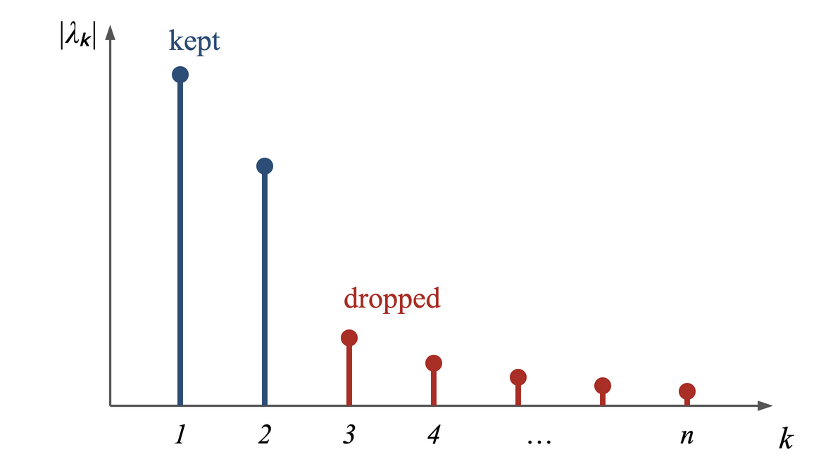
This form suggests an approximation. Number the eigenvalues so that \(|\lambda_1| \geq |\lambda_2| \geq \cdots \geq |\lambda_n|\). If the first few are much larger in size than the rest, as in Figure 3, the terms with small \(|\lambda_k|\) can be dropped. For instance, when \(|\lambda_3|,\ldots,|\lambda_n|\) are much smaller than \(|\lambda_1|\) and \(|\lambda_2|\), keeping two terms gives
A bound on the error can be read off from (17). The part dropped is \(E = \lambda_3q_3q_3^T + \cdots + \lambda_nq_nq_n^T\). A unit vector has entries of size at most \(1\), so every entry of each \(q_kq_k^T\) has size at most \(1\), and every entry of \(E\) has size at most \(|\lambda_3| + \cdots + |\lambda_n|\). The approximation also needs far less storage: two numbers and two vectors, \(2n + 2\) numbers in all, in place of the \(n^2\) entries of \(A\).
12. Unitary matrices
Section 11 gave a name to the complex counterpart of an orthogonal matrix. A square complex matrix \(U\) is unitary if
that is, if its columns are orthonormal in \(\mathbb{C}^n\): the \((k,l)\) entry of \(U^HU\) is \(u_k^Hu_l\), where \(u_k\) is column \(k\). A real unitary matrix is an orthogonal matrix in the sense of Chapter 3. As there, the condition is needed only one way round. Since \(U\) is square, \(U^HU = I\) gives \(U^{-1} = U^H\) (Step 3 of the proof of Theorem 5.8), so \(UU^H = I\) as well, and the rows of \(U\) are orthonormal too. The matrix has to be square for this. A tall \(m\times n\) matrix with orthonormal columns also has \(U^HU = I\), but then \(UU^H\) is \(m\times m\) with rank at most \(n < m\), so it cannot be the identity (Chapter 3 made the same point for a tall real \(Q\)).
Theorem 5.19. Let \(U\) be an \(n\times n\) unitary matrix. Then:
-
\((Ux)^H(Uy) = x^Hy\) for all \(x, y \in \mathbb{C}^n\), and in particular \(\|Ux\| = \|x\|\);
-
every eigenvalue \(\lambda\) of \(U\) has \(|\lambda| = 1\);
-
eigenvectors of \(U\) belonging to distinct eigenvalues are orthogonal: if \(Ux_1 = \lambda_1x_1\) and \(Ux_2 = \lambda_2x_2\) with \(\lambda_1 \neq \lambda_2\), then \(x_1^Hx_2 = 0\).
Proof
Part 1. By the product rule for \({}^H\) (Section 11), \((Ux)^H(Uy) = x^HU^HUy = x^Hy\). Taking \(y = x\) gives \(\|Ux\|^2 = \|x\|^2\). This is Theorem 3.15 of Chapter 3 with \({}^H\) in place of \({}^T\).
Part 2. Let \(Ux = \lambda x\) with \(x \neq 0\). By Part 1,
and \(\|x\| > 0\), so \(|\lambda| = 1\).
Part 3. By Part 1, and then the rule \((cx)^H = \overline{c}\,x^H\),
so \((1 - \overline{\lambda_1}\lambda_2)\,x_1^Hx_2 = 0\). By Part 2, \(\overline{\lambda_1}\lambda_1 = |\lambda_1|^2 = 1\). If \(\overline{\lambda_1}\lambda_2\) were also \(1\), then \(\overline{\lambda_1}(\lambda_2 - \lambda_1) = 0\), and since \(\overline{\lambda_1} \neq 0\) this would force \(\lambda_2 = \lambda_1\). So \(1 - \overline{\lambda_1}\lambda_2 \neq 0\), and \(x_1^Hx_2 = 0\).
Part 2 does not say that \(\lambda = \pm 1\). Those are the only real numbers of size \(1\), but the eigenvalues of a unitary matrix can be complex, and Part 2 only says that they lie on the unit circle of the complex plane. The comparison with Theorem 5.16 is direct: the eigenvalues of a Hermitian matrix lie on the real line, those of a unitary matrix on the unit circle. Part 3 has the same form as Part 3 of Theorem 5.16, with the same restriction to distinct eigenvalues.
12.1. Rotations and the Fourier matrix
Rotations. The rotation of the plane through an angle \(\theta\),
is real with orthonormal columns, so it is orthogonal, and hence unitary. Its characteristic polynomial is \((\cos\theta - \lambda)^2 + \sin^2\theta\), whose roots are \(\lambda = \cos\theta \pm j\sin\theta = e^{\pm j\theta}\), both of size \(1\). Take \(\sin\theta \neq 0\) (otherwise \(R_\theta = \pm I\)). For \(\lambda = e^{j\theta}\), the first row of \(R_\theta - \lambda I\) is \((-j\sin\theta,\ -\sin\theta)\), so an eigenvector \((x_1,x_2)\) has \(x_2 = -jx_1\); for \(e^{-j\theta}\) the same step gives \(x_2 = jx_1\). So
The matrix \(R\) of Section 3.4 is the case \(\theta = 90^\circ\), with eigenvalues \(\pm j\) (Section 3.4 scaled the eigenvectors to \((j,1)\) and \((j,-1)\), which are \(j\) times these). The two eigenvalues are distinct, and as Part 3 requires, \(x^Hy = 1\cdot 1 + \overline{(-j)}\,j = 1 + j^2 = 0\). Without the conjugate the answer would be \(x^Ty = 1 + (-j)(j) = 2\). The plain transpose would also give \(x^Tx = 1 + (-j)^2 = 0\) for the nonzero vector \(x\), so it cannot serve as a squared length; this is the reason Chapter 3 gave for the conjugate in \(x^Hx\), using the same vector \((1,j)\). Dividing each vector by \(\sqrt2\) makes the pair orthonormal.
The Fourier matrix. Let \(w = e^{2\pi j/n}\), the point on the unit circle at angle \(2\pi/n\). Its powers \(1, w, \ldots, w^{n-1}\) are the \(n\) distinct \(n\)-th roots of \(1\), spaced evenly round the circle. The Fourier matrix \(F\) is the \(n\times n\) matrix with entries \(F_{kl} = w^{kl}\), with rows and columns numbered from \(0\) to \(n-1\):
The claim is that \(U = F/\sqrt n\) is unitary. Column \(l\) of \(F\) is \(f_l = (1, w^l, w^{2l}, \ldots, w^{(n-1)l})^T\). Since \(|w| = 1\), \(\overline{w} = 1/w\), so \(\overline{w^{mk}} = w^{-mk}\) and
If \(l = k\), every term is \(1\) and the sum is \(n\). If \(l \neq k\), put \(z = w^{l-k}\). Now \(w^p = e^{2\pi jp/n}\) equals \(1\) only when \(p\) is a multiple of \(n\), and \(0 < |l-k| < n\), so \(z \neq 1\), while \(z^n = (w^n)^{l-k} = 1\). The sum is geometric:
So \(F^HF = nI\), and \(U = F/\sqrt n\) has \(U^HU = I\). For \(n = 4\), \(w = e^{j\pi/2} = j\), and
for instance \(f_0^Hf_1 = 1 + j - 1 - j = 0\) and \(f_1^Hf_1 = 1 + (-j)(j) + (-1)(-1) + (j)(-j) = 4\).
13. Similar matrices
Diagonalization (Section 6) turned \(A\) into \(\Lambda = S^{-1}AS\) with the eigenvector matrix \(S\). The same operation can be carried out with any invertible matrix in place of \(S\). Square matrices \(A\) and \(B\) are called similar if
The relation works both ways: \(A = MBM^{-1}\), which is (20) with the roles of \(A\) and \(B\) exchanged and \(M^{-1}\) in place of \(M\). In this language, the definition of Section 6 reads: \(A\) is diagonalizable if it is similar to a diagonal matrix. The class gave three uses of similarity.
13.1. A change of variables in a recursion
Take the recursion \(u_k = Au_{k-1}\) of Section 10, and introduce new variables \(v_k\) through \(u_k = Mv_k\), with \(M\) a fixed invertible matrix. Nothing is lost, since \(v_k = M^{-1}u_k\). Substituting,
The recursion for the new variables has the similar matrix \(B\) in place of \(A\), and \(u_k = MB^kv_0\). If \(B\) is simpler than \(A\), the work moves to \(B\). Section 10 is the case \(M = S\), \(B = \Lambda\): there \(v_0\) was the coefficient vector \(c = S^{-1}u_0\), and \(\Lambda^k\) acted on it entry by entry.
13.2. Similar matrices have the same eigenvalues
Lemma 5.7, stated with \(S\) in place of \(M\), already shows that \(M^{-1}AM\) has the same characteristic polynomial as \(A\), and so the same eigenvalues with the same algebraic multiplicities. The eigenvectors are not the same, but they correspond through \(M\).
Theorem 5.20. Let \(B = M^{-1}AM\) with \(M\) invertible. If \(Ax = \lambda x\) with \(x \neq 0\), then \(M^{-1}x \neq 0\) and \(B(M^{-1}x) = \lambda(M^{-1}x)\). Conversely, if \(Bz = \lambda z\) with \(z \neq 0\), then \(Mz \neq 0\) and \(A(Mz) = \lambda(Mz)\).
Proof
Substitute \(A = MBM^{-1}\) into \(Ax = \lambda x\) to get \(MBM^{-1}x = \lambda x\), and multiply on the left by \(M^{-1}\): \(B(M^{-1}x) = \lambda M^{-1}x\). If \(M^{-1}x\) were \(0\), then \(x = M(M^{-1}x) = 0\), which it is not. So \(\lambda\) is an eigenvalue of \(B\) with eigenvector \(M^{-1}x\). For the converse, \(A(Mz) = MBM^{-1}Mz = MBz = \lambda Mz\), and \(Mz \neq 0\) because \(M\) is invertible and \(z \neq 0\).
13.3. Change of basis
Let \(\mathcal{X} = \{x_1,\ldots,x_n\}\) and \(\mathcal{Y} = \{y_1,\ldots,y_n\}\) be two bases of \(\mathbb{C}^n\), and let \(X\) and \(Y\) be the matrices with these vectors as columns; both are invertible. Each \(y_l\) is a combination of the \(x\)'s, \(y_l = Xm_l\), where \(m_l = [y_l]_{\mathcal{X}}\) is its coordinate column in the basis \(\mathcal{X}\) (in the bracket notation of Chapter 2). Putting the \(n\) columns side by side,
and \(M = X^{-1}Y\) is invertible. Now take a vector \(v\), with coordinate columns \(\alpha = [v]_{\mathcal{X}}\) and \(\beta = [v]_{\mathcal{Y}}\). Then \(v = X\alpha = Y\beta = XM\beta\), and since \(X\) is invertible,
The same matrix appears twice but works in opposite directions. In (21) it builds the new basis vectors out of the old ones; in (22) it turns coordinates in the new basis into coordinates in the old one. In the language of Chapter 2, \(M\) is the matrix of the identity map, with input basis \(\mathcal{Y}\) and output basis \(\mathcal{X}\).
Similarity enters when a linear transformation is written in the two bases. Suppose \(T\) has matrix \(A\) in the basis \(\mathcal{X}\), meaning \([Tv]_{\mathcal{X}} = A[v]_{\mathcal{X}}\) for every \(v\). Using (22) twice,
So in the basis \(\mathcal{Y}\) the same transformation has the matrix
The matrices of one transformation in two bases are similar. This is the computation of the recursion above, read differently: there \(u_k = Mv_k\) was a change of variables, here \(\alpha = M\beta\) is a change of coordinates.
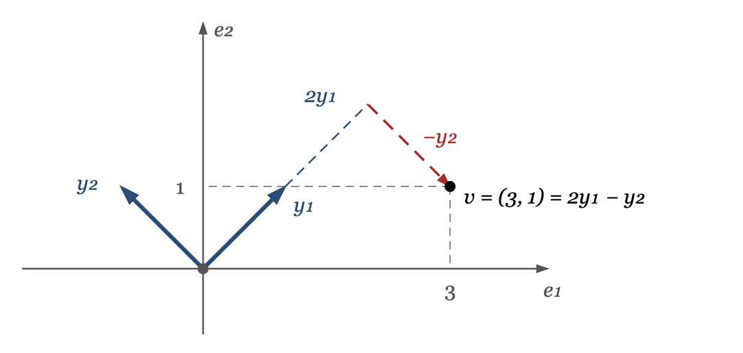
An example. In \(\mathbb{R}^2\) take \(\mathcal{X}\) to be the standard basis, so \(X = I\), and \(y_1 = (1,1)\), \(y_2 = (-1,1)\). Then \(M = Y\) and
The vector \(v = (3,1)\) has \(\alpha = (3,1)\) and \(\beta = M^{-1}\alpha = \tfrac12(4,-2) = (2,-1)\); indeed \(2y_1 - y_2 = (3,1)\) (Figure 4). Next take \(T\) to be the projection onto the line through \(y_1\). In the standard basis its matrix is \(P = y_1y_1^T/(y_1^Ty_1)\) (Chapter 3):
Since \(Py_1 = y_1\) and \(Py_2 = 0\), \(PM = [y_1\ \ 0]\), and \(M^{-1}y_1 = e_1\) because \(y_1\) is the first column of \(M\). So
This is the matrix \(P'\) that Chapter 2, in The matrix depends on the basis, wrote down by describing the projection in a basis adapted to it; (23) now produces it by calculation. The two matrices have the same eigenvalues, \(1\) and \(0\), as Lemma 5.7 says, and the eigenvector \(y_1\) of \(P\) corresponds to the eigenvector \(M^{-1}y_1 = e_1\) of \(P'\), as Theorem 5.20 says.