Companion page: Chapter 1 Matlab resources — commands for trying out the material below on a machine.
Almost the whole of this course is built around two equations. The first is \(Ax=b\), and the second is \(Ax=\lambda x\). This chapter is about the first one. The questions we want to answer are: when does a solution exist, when is it unique, how do we compute it, and how much does that computation cost. The last question matters as much as the others. In engineering practice the matrices are large, the arithmetic is done in finite precision, and an algorithm that is correct on paper can still give you a badly wrong answer on a machine.
The reference for this material is Chapter 1 of Gilbert Strang (GS). The book is a good place to see the mechanics. Here we will be a little more careful than the book about what is being claimed and why it is true, and we will not repeat an idea with several numerical examples when one will do.
1. Notation
A few conventions that we will follow throughout the course.
-
Upper case letters (\(A, B, U, L\)) denote matrices, lower case letters (\(x, b, \lambda\)) denote vectors and scalars. The context will make it clear which of the two a lower case letter is.
-
A vector \(x \in \mathbb{R}^n\) is a column by default. A row vector is written as \(x^T\).
-
\(A_{ij}\) (or \(a_{ij}\)) is the entry of \(A\) in row \(i\) and column \(j\). Row index first, always.
-
\(a_j\) denotes the \(j\)-th column of \(A\), and \(e_j\) denotes the \(j\)-th column of the identity matrix.
-
We will work over the real numbers \(\mathbb{R}\) most of the time, and switch to the complex numbers \(\mathbb{C}\) when we get to eigenvalue problems.
An \(m \times n\) matrix \(A\) and a vector \(b \in \mathbb{R}^m\) together define the system \(Ax=b\), which is \(m\) equations in \(n\) unknowns. Written out,
There are two useful ways to read this: one equation at a time (the row picture), or one column at a time (the column picture). Both are useful, because they answer different questions.
2. The row picture
2.1. Describing a plane
Take a single equation, say \(5x + 6y + 3z = 7\). You know from school that this is a plane in three dimensions. Let us derive that fact properly, because the derivation generalizes to \(n\) dimensions without any change.
A plane is fixed by two pieces of data: the direction perpendicular to it, given by a unit normal \(\hat{n}\), and how far it sits from the origin, given by a distance \(d\). Drop a perpendicular from the origin \(O\) onto the plane and call the foot \(N\). Then \(\vec{ON} = d\,\hat{n}\). Now take any point \(P\) on the plane with position vector \(\vec{r}\). The segment \(\vec{NP} = \vec{r} - d\,\hat{n}\) lies entirely within the plane, so it must be perpendicular to \(\hat{n}\).
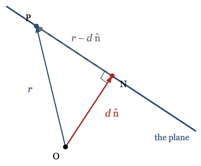
Writing that perpendicularity as a dot product,
For \(d \neq 0\) this gives \(\vec{r}\cdot\hat{n} = d\). (When \(d=0\) the plane passes through the origin and \(\vec{r}\cdot\hat{n}=0\) holds directly, so the relation \(\vec{r}\cdot\hat{n}=d\) covers every case.) With \(\vec{r}=(x,y,z)\) and \(\hat{n}=(n_x,n_y,n_z)\) this is
Two points about this equation. First, an equation and any nonzero multiple of it describe the same plane, so the coefficients by themselves do not fix \(\hat{n}\) and \(d\) — you must normalize before you read the right hand side as a distance. For \(5x+6y+3z=7\) we have \(\hat{n} = (5,6,3)/\sqrt{70}\) and \(d = 7/\sqrt{70}\). Second, if you want \(d\) to be a genuine (non-negative) distance and the arithmetic hands you \(d<0\), simply absorb the sign into \(\hat{n}\); the normal then points the other way.
Nothing in the argument used the number three. In \(\mathbb{R}^n\), with \(\vec{r}=(x_1,\ldots,x_n)\) and \(\hat{n}=(a_1,\ldots,a_n)\), the same steps give
and the solution set is called a hyperplane: a flat object of dimension \(n-1\) sitting inside \(n\) dimensions. One scalar equation removes exactly one degree of freedom.
Why is the dimension exactly \(n-1\), and not less?
Let \(a \neq 0\) and let \(S = \{x : a^Tx = d\}\). Pick any particular solution \(x_p\) (for instance \(x_p = d\,a/\|a\|^2\)). Then \(x \in S\) if and only if \(a^T(x - x_p) = 0\), i.e. \(S = x_p + N\) where \(N = \{v : a^Tv = 0\}\). So \(S\) is the set \(N\) shifted by a fixed vector, and it has the same dimension as \(N\).
Now \(N\) is the set of vectors orthogonal to \(a\). Complete \(a/\|a\|\) to an orthonormal basis \(\{a/\|a\|, u_2,\ldots,u_n\}\) of \(\mathbb{R}^n\). Writing \(v\) in this basis, \(a^Tv=0\) kills exactly the first coordinate and leaves the other \(n-1\) free. Hence \(\dim N = n-1\). We will make the words "basis" and "dimension" precise in the next chapter; for now the counting argument is the thing to hold on to.
2.2. A system as an intersection of hyperplanes
With this, \(Ax=b\) with \(A\) of size \(n\times n\) is a set of \(n\) hyperplanes in \(\mathbb{R}^n\), row \(i\) giving the hyperplane \(\sum_j a_{ij}x_j = b_i\). A solution is a point lying on all of them at once. So solving the system means intersecting \(n\) hyperplanes.
In two dimensions this is two lines in a plane, and there are only three things that can happen: they cross at one point, they are parallel and distinct, or they are the same line.
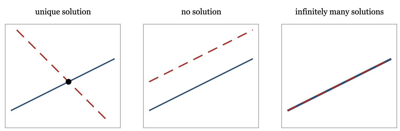
In three dimensions the arrangements are richer — three planes can meet at a point, meet along a common line, form a triangular prism with no common point, be parallel, and so on — but the outcomes are still only three in number, and there is a reason for that.
Claim 1.1. For a system \(Ax=b\) over \(\mathbb{R}\), the number of solutions is either zero, exactly one, or infinite. It can never be, say, exactly two.
Proof
Suppose \(x_1 \neq x_2\) are both solutions, so \(Ax_1 = Ax_2 = b\). For any scalar \(t \in \mathbb{R}\) consider \(x_t = x_1 + t(x_2 - x_1)\). By linearity,
\(A x_t = Ax_1 + t(Ax_2 - Ax_1) = b + t(b - b) = b .\)
So every \(x_t\) is a solution. Since \(x_2 - x_1 \neq 0\) and \(t\) ranges over the infinitely many reals, these \(x_t\) are all distinct. Hence two distinct solutions force infinitely many. The three cases follow.
The cases with no solution or with infinitely many are lumped together and called the singular case. The word will be given a sharper meaning shortly, once we have elimination and pivots in hand.
A remark on why the case of no solution is the common one in practice. In an experiment you typically measure more quantities than you have unknowns, so \(A\) is tall (\(m > n\)), and each measurement is corrupted by noise. The hyperplanes then fail to have a common point by a small amount. Insisting on an exact solution is the wrong thing to ask for; what one wants is the point that misses all of them by as little as possible. That is the least squares problem, and we do it properly in the chapter on orthogonality.
3. The column picture
Now read the same equation column-wise. Split \(A\) into its columns \(a_1,\ldots,a_n\), and observe that
Check this by comparing the \(i\)-th entry on both sides. So \(Ax\) is nothing but a weighted sum of the columns of \(A\), with the entries of \(x\) supplying the weights. Such a weighted sum is called a linear combination. The system \(Ax=b\) is therefore asking a different-sounding question:
Can \(b\) be written as a linear combination of the columns of \(A\), and if so, in how many ways?
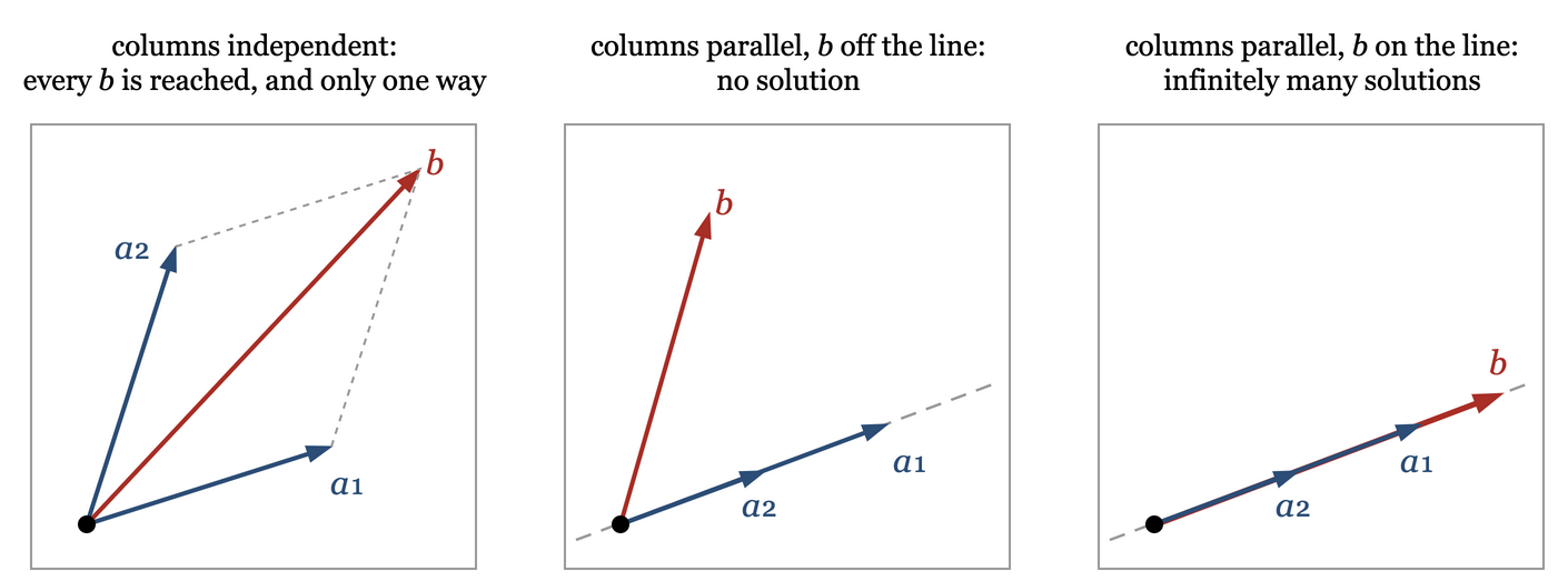
The two questions have separated cleanly, and that is what the column picture gives us:
-
Existence of a solution is about \(b\): is it reachable from the columns at all? The set of all reachable vectors is called the column space of \(A\).
-
Uniqueness is about \(A\) alone, and has nothing to do with \(b\): are the columns independent, or is one of them redundant?
The claim that the second question does not involve \(b\) needs a proof.
Claim 1.2. \(Ax=b\) has at most one solution for every \(b\) if and only if \(Ax=0\) implies \(x=0\).
Proof
(\(\Rightarrow\)) Take \(b=0\). Since \(x=0\) is always a solution of \(Ax=0\), uniqueness forces it to be the only one.
(\(\Leftarrow\)) Suppose \(Ax_1 = Ax_2 = b\). Then \(A(x_1-x_2)=0\), so by hypothesis \(x_1-x_2=0\).
So the question of uniqueness reduces to studying \(Ax=0\), which is a statement about the columns of \(A\) only. In three dimensions the failure mode is easy to picture: if the three columns happen to lie in a common plane, then no \(b\) outside that plane can be reached at all, and any \(b\) that is reachable is reachable in infinitely many ways. This is the vector space language that Chapter 2 builds up carefully.
4. Gaussian elimination
Pictures tell us what to expect. To actually get \(x\) we need an algorithm, and the one everybody uses is elimination, which you have seen in school. What we want out of it here is threefold: a clean statement of the algorithm, a clear account of when it breaks down, and an honest estimate of its cost.
4.1. Forward elimination and back substitution
Take the system
Subtract \(2\times\) row 1 from row 2, and \((-1)\times\) row 1 from row 3, so as to create zeros below the leading \(2\). Then subtract \((-1)\times\) the new row 2 from the new row 3. Carrying the right hand side along, the augmented array goes
The entries \(2, -8, 1\) that sit at the head of each row at the moment it is used are the pivots, and this stage is called forward elimination. The matrix is now upper triangular, and the system can be read off from the bottom up: \(w=2\), then \(-8v-2(2)=-12\) gives \(v=1\), then \(2u+1+2=5\) gives \(u=1\). This stage is back substitution, and the solution is \((1,1,2)\).
In general, at step \(k\) we use row \(k\) to clear column \(k\) in all the rows below it. Denoting by \(a^{(k)}_{ij}\) the entries at the start of step \(k\), the algorithm is
for \(k = 1,\ldots,n-1\). The numbers \(\ell_{ik}\) are called the multipliers, and \(a^{(k)}_{kk}\) is the \(k\)-th pivot. Keep the multipliers in mind — they are about to reappear, arranged in a matrix.
4.2. When elimination breaks down
The algorithm divides by the pivot, so a zero in the pivot position stops it. Two rather different things can be happening.
The first is a nuisance rather than a real problem. In
the second pivot is zero, but there is a nonzero entry below it in the same column. Exchanging rows 2 and 3 restores the elimination, and the system is perfectly well behaved. The zero was an artefact of the order in which the equations happened to be written down.
The second is genuine trouble. If in the same column every entry from the pivot position downwards is zero, no exchange can help. Then the matrix is singular in the sense of the previous section, and depending on the right hand side we get either no solution or infinitely many. Let us see this happen inside the elimination.
Change one entry so that no exchange can help: run elimination on \(\begin{bmatrix} 1 & 1 & 1 \\ 2 & 2 & 5 \\ 4 & 4 & 8\end{bmatrix}\) and find right hand sides producing each of the two singular outcomes.
Subtracting \(2\times\) row 1 from row 2 and \(4\times\) row 1 from row 3 gives
Now column 2 is entirely zero below the pivot position, and no exchange can produce a second pivot — this is the genuine trouble. The last two rows say \(3w = b_2-2b_1\) and \(4w = b_3-4b_1\), two equations in the single unknown \(w\).
Take \(b = (0,6,8)\). Then \(3w=6\) and \(4w=8\) both give \(w=2\), so the two equations agree. Row 1 now reads \(u+v+w = 0\), i.e. \(u+v = -2\), and this one equation in two unknowns can be satisfied in infinitely many ways — \(v\) is free, with \(u = -2-v\). So the system has infinitely many solutions.
Take \(b = (0,3,5)\) instead. Then \(3w=3\) gives \(w=1\) while \(4w=5\) gives \(w=1.25\). The equations are inconsistent, and there is no solution at all.
The same singular matrix therefore gives either outcome, decided entirely by \(b\). This is the row picture’s "no solution" and "infinitely many solutions" showing up as arithmetic.
The two look alike in the middle of a calculation, so we state the test that separates them carefully.
|
Important
|
Singularity is decided by the pivots we can finally produce, not by the zeros we meet on the way. A zero in a pivot position is by itself no cause for alarm: the matrix \(\begin{bmatrix} 0 & 1 \\ 1 & 0\end{bmatrix}\) has one in the very first pivot position and is perfectly invertible, since a single row exchange fixes it. The statement to hold on to is: \(A\) is singular exactly when, even after row exchanges, fewer than \(n\) nonzero pivots can be produced. |
4.3. The cost of elimination
For a \(3\times 3\) system nobody cares about cost. For \(n = 10^6\), which is a routine size in engineering computation, cost is the only thing one cares about. Let us count.
At step \(k\) there are \(n-k\) rows below the pivot row. For each of them we compute one multiplier (a division), and then update the entries in columns \(k+1\) through \(n\) — that is \(n-k\) entries, each needing one multiplication and one subtraction. The entry in column \(k\) itself is set to zero and costs nothing. So step \(k\) costs \((n-k)\) divisions and \((n-k)^2\) multiply-subtract pairs, and the total over all steps is
multiply-subtract pairs, plus \(n(n-1)/2 \approx n^2/2\) divisions. The leading behaviour is what matters: elimination on the matrix costs \(O(n^3)\), and more precisely about \(n^3/3\) operations.
The right hand side is far cheaper. Carrying \(b\) through forward elimination costs \(n-k\) operations at step \(k\), i.e. \(n(n-1)/2\) in all, and back substitution costs about the same. So
|
Note
|
Working on the matrix costs \(\sim n^3/3\) operations. Working on each right hand side costs \(\sim n^2\) operations. The gap between \(n^3\) and \(n^2\) is the main point of this chapter, and the LU decomposition below is built to exploit it. |
Estimate the cost of back substitution alone, carefully.
To find \(x_n\) from \(u_{nn}x_n = c_n\) takes 1 division. To find \(x_i\) we compute \(x_i = \left(c_i - \sum_{j>i} u_{ij}x_j\right)/u_{ii}\), which needs \(n-i\) multiply-subtract pairs and 1 division. Summing over \(i=1,\ldots,n\) gives \(\sum_{i=1}^n (n-i) = n(n-1)/2\) multiply-subtract pairs and \(n\) divisions, i.e. about \(n^2/2\) operations.
Is \(n^3\) the end of the story? Ordinary matrix multiplication is also an \(O(n^3)\) operation, and Strassen showed in 1969 that it can be done in \(O(n^{\log_2 7}) = O(n^{2.81})\); later theoretical constructions have pushed the exponent below \(2.38\), though those algorithms have enormous constants and are never used in practice. Solving a linear system can be made to run at the same exponent as matrix multiplication. In practice, for dense matrices, \(n^3/3\) is what you get. The real savings come from a different direction — from the structure of \(A\), which is the subject of the last section of this chapter.
5. Inner and outer products
Before writing elimination in matrix language we need two pieces of notation that will be used for the rest of the course. Let \(x, y \in \mathbb{R}^n\).
The inner product (also written \(\langle x,y\rangle\) or \((x,y)\)) multiplies a \(1\times n\) by an \(n \times 1\) and produces a scalar:
The outer product multiplies an \(n\times 1\) by a \(1 \times n\) and produces a matrix:
The outer product is a very special matrix. It is built out of \(2n\) numbers but has \(n^2\) entries, so it is enormously redundant; every one of its columns is a multiple of \(x\). Matrices of this form are said to have rank one, and they are the atoms out of which general matrices are assembled. Indeed, if \(C = AB\) with \(A\) of size \(m\times p\) and \(B\) of size \(p\times n\), then besides the familiar entry-by-entry rule \(C_{ij} = \sum_k A_{ik}B_{kj}\), we may write
where \(a_k\) is column \(k\) of \(A\) and \(b_k^T\) is row \(k\) of \(B\). Verify it by comparing the \((i,j)\) entries: the right hand side gives \(\sum_k (a_k)_i (b_k^T)_j = \sum_k A_{ik}B_{kj}\), as required. We will meet this outer product form again, and centrally, when we do the singular value decomposition.
6. Elimination as matrix multiplication
We now ask: can a step of Gaussian elimination be written as multiplication by a matrix? The motivation is not aesthetic. If each step is a matrix, then the whole elimination is a product of matrices, and we can ask what that product is — which is exactly how the LU decomposition falls out.
6.1. Elementary matrices
Start from \(IA = A\) and modify \(I\) a little. Define, for \(i \neq k\),
which is the identity with the single extra entry \(-\ell\) in position \((i,k)\). Then
and since \(e_i\) times a row vector places that row in position \(i\) and zeros elsewhere, the effect is precisely \(\text{row}_i \leftarrow \text{row}_i - \ell\,\text{row}_k\). These are called elementary or elimination matrices. Note that \(i>k\) for our purposes (we always subtract an earlier row from a later one), so \(E_{ik}\) is lower triangular with ones on the diagonal — unit lower triangular, in the standard phrase.
6.2. Commuting elementary matrices
Elimination on a \(3\times3\) matrix uses \(E_{21}\), \(E_{31}\) and then \(E_{32}\). It is natural to ask whether the order matters. The outer product form answers this in one line. Using \((e_a e_b^T)(e_c e_d^T) = (e_b^Te_c)\, e_a e_d^T\) and \(e_b^Te_c = \delta_{bc}\),
So the two commute exactly when \(\delta_{kj} = \delta_{mi} = 0\), i.e. when neither operation touches a row that the other one uses. \(E_{21}\) and \(E_{31}\) commute, because both of them modify rows using row 1 and neither of them modifies row 1. But \(E_{32}\) and \(E_{21}\) do not commute, because \(E_{21}\) changes row 2 which \(E_{32}\) then uses. This is exactly the intuition you would have from doing elimination by hand, now made precise.
6.3. Inverses of elementary matrices
The inverse of \(E_{ik}(\ell)\) must undo the row operation, i.e. it must add back what was subtracted. So we expect \(E_{ik}(\ell)^{-1} = E_{ik}(-\ell) = I + \ell\,e_ie_k^T\). The algebra confirms it:
since \(e_k^Te_i = 0\) for \(i \neq k\). So to invert an elementary matrix we only flip the sign of its off-diagonal entry.
6.4. Products and inverses of triangular matrices
Two facts we will keep using.
Lemma 1.3. The product of two lower triangular matrices is lower triangular. If both have unit diagonal, so does the product.
Proof
Let \(P,Q\) be lower triangular, so \(P_{ik}=0\) for \(i<k\) and \(Q_{kj}=0\) for \(k<j\). For \(M = PQ\) and any \(i<j\),
In the first sum \(k<j\) forces \(Q_{kj}=0\). In the second sum \(k \geq j > i\) forces \(P_{ik}=0\). So \(M_{ij}=0\) whenever \(i<j\), i.e. \(M\) is lower triangular. For the diagonal, \(M_{ii} = \sum_k P_{ik}Q_{ki}\), and the same two conditions leave only \(k=i\), giving \(M_{ii}=P_{ii}Q_{ii}\). Hence unit diagonals multiply to a unit diagonal.
Lemma 1.4. A lower triangular matrix with nonzero diagonal entries is invertible, and its inverse is lower triangular, with unit diagonal if the original had one.
Proof
Let \(L\) be lower triangular with nonzero diagonal entries. For each \(j\), forward substitution solves \(Lx = e_j\) uniquely — at every step it divides by a diagonal entry, which is nonzero — so \(L\) has an inverse, its \(j\)th column being that \(x\). Fix \(j\) and look at that column. Forward substitution reads \(L_{11}x_1 = 0,\; L_{21}x_1 + L_{22}x_2 = 0,\ \ldots\), and as long as we are above row \(j\) the right hand side is zero, so \(x_1 = \cdots = x_{j-1} = 0\). Since column \(j\) of \(L^{-1}\) is exactly this \(x\), all entries of \(L^{-1}\) above the diagonal vanish. Row \(j\) then gives \(L_{jj}x_j = 1\), so \((L^{-1})_{jj} = 1/L_{jj}\), which is 1 when \(L_{jj}=1\).
Taken together, the unit lower triangular matrices are closed under products and inverses. Everything we are about to do stays inside this family.
7. The LU decomposition
Forward elimination on a \(3\times3\) matrix, with no row exchanges, is the sequence \(E_{21}\), \(E_{31}\), \(E_{32}\), so that
with \(U\) upper triangular. Multiplying by the inverses in the reverse order,
By Lemma 1.3, \(L\) is unit lower triangular. But something much better than that is true: the multipliers appear in \(L\) in place, with no sign changes and no arithmetic at all. For the \(3\times3\) case,
The book asks you to accept this after looking at an example. We shall prove it; the outer product notation makes the argument short.
Prove that the multipliers land in \(L\) unchanged, for general \(n\).
With the standard ordering (clear column 1 top to bottom, then column 2, and so on), we have
the factors taken left to right in increasing \(k\), and within a given \(k\) in increasing \(i\). Expanding the product, a cross term between a factor \((i,k)\) and a later factor \((i',k')\) carries the coefficient \(e_k^Te_{i'} = \delta_{ki'}\), so it survives only if \(k = i'\). But "later" means either \(k' > k\), or \(k'=k\) with \(i'>i\); in both cases \(k' \geq k\). Combined with \(i' > k'\) (the factors are strictly below the diagonal) and \(k=i'\), we would need \(k = i' > k' \geq k\), which is impossible. So every cross term vanishes and
\(L = I + \sum_{i>k} \ell_{ik}\,e_ie_k^T ,\)
which is exactly the statement that \(\ell_{ik}\) sits in position \((i,k)\). (A product of three or more of the factors dies for the same reason: it already contains the contraction between its first two.)
So elimination already produces the factorization: run forward elimination, store the multipliers in the space that the zeros vacated, and you have \(L\) and \(U\) with no work beyond the elimination itself.
7.1. Using the factorization
Given \(A = LU\), the system \(Ax=b\) becomes \(L(Ux)=b\), and is solved in two triangular sweeps:
-
Solve \(Lc = b\) for \(c\) by forward substitution (\(c_1\) first, then \(c_2\), and so on).
-
Solve \(Ux = c\) for \(x\) by back substitution (\(x_n\) first, then \(x_{n-1}\), and so on).
Each sweep costs \(O(n^2)\). Now recall the cost gap noted earlier. The factorization is done once, at \(\sim n^3/3\). After that, every new right hand side costs only \(\sim n^2\). In engineering this is the common situation: the same physical system (same \(A\)) is driven by many different sources (many \(b\)). Factor once, solve many times.
7.2. The LDU form
The pivots sit on the diagonal of \(U\). Pulling them out into a diagonal matrix \(D = \mathrm{diag}(d_1,\ldots,d_n)\) and dividing each row of \(U\) by its pivot leaves an upper triangular matrix with ones on the diagonal:
This gives \(A = LDU\), now with both triangular factors carrying unit diagonals and all the scaling collected in \(D\). The symmetry of the notation is the point: \(L\) and \(U\) are on the same footing, which is what makes the next result possible.
7.3. Uniqueness of the factorization
Theorem 1.5. Let \(A\) be nonsingular and suppose \(A = L_1D_1U_1 = L_2D_2U_2\), where the \(L_i\) are unit lower triangular, the \(U_i\) are unit upper triangular and the \(D_i\) are diagonal with no zero on the diagonal. Then \(L_1=L_2\), \(D_1=D_2\) and \(U_1=U_2\).
The book states this and moves on. Here is the proof; it is short, and we will need it in a moment for symmetric matrices.
Proof
From \(L_1D_1U_1 = L_2D_2U_2\), multiply on the left by \(L_2^{-1}\) and on the right by \(U_1^{-1}\):
\(L_2^{-1}L_1D_1 = D_2U_2U_1^{-1} .\)
Look at the two sides separately. By Lemmas 1.3 and 1.4, \(L_2^{-1}L_1\) is unit lower triangular, and multiplying on the right by a diagonal matrix scales columns, so the left hand side is lower triangular with diagonal entries equal to those of \(D_1\). By the same lemmas applied to upper triangular matrices, the right hand side is upper triangular with diagonal entries equal to those of \(D_2\).
A matrix that is simultaneously lower and upper triangular is diagonal. Call it \(M\). Reading off the diagonals gives \(M = D_1 = D_2\). Then \(L_2^{-1}L_1 D_1 = D_1\) with \(D_1\) invertible gives \(L_2^{-1}L_1 = I\), i.e. \(L_1 = L_2\). Similarly \(U_2U_1^{-1} = I\), so \(U_1 = U_2\).
7.4. Existence of the factorization
We assumed no row exchanges were needed. That assumption is not free, and it can be characterized exactly. Write \(A_k\) for the leading principal submatrix of \(A\), i.e. the top-left \(k\times k\) block.
Theorem 1.6. Gaussian elimination on \(A\) produces \(n\) nonzero pivots without any row exchanges if and only if \(A_k\) is nonsingular for every \(k=1,\ldots,n\). In that case \(A=LU\) exists and, by Theorem 1.5, is unique.
Proof
Suppose elimination has completed \(k-1\) steps without a row exchange. Each step was a multiplication by a unit lower triangular matrix, so the current array is \(A^{(k)} = MA\) with \(M\) unit lower triangular.
The key observation is that leading blocks multiply on their own. For \(i,j\leq k\), \((MA)_{ij} = \sum_l M_{il}A_{lj}\), and \(M_{il}=0\) for \(l>i\), so the sum runs only over \(l \leq i \leq k\). Hence
\(\left(A^{(k)}\right)_k = M_k A_k ,\)
where the subscript \(k\) denotes the leading \(k\times k\) block. Now \(M_k\) is unit lower triangular, hence nonsingular, and so \(A_k\) is nonsingular exactly when \(\left(A^{(k)}\right)_k\) is. Also \(\left(A^{(k)}\right)_k\) is upper triangular — columns \(1\) through \(k-1\) have already been cleared below the diagonal, and whatever is left of column \(k\) below the diagonal lies in rows past \(k\), outside this block — with diagonal entries \(d_1,\ldots,d_{k-1}\) (the pivots already produced) followed by \(a^{(k)}_{kk}\), the candidate for the \(k\)-th pivot.
It remains to connect that diagonal to nonsingularity, in both directions. If all of \(d_1,\ldots,d_{k-1},a^{(k)}_{kk}\) are nonzero, then \(\left(A^{(k)}\right)_k\) is invertible by (the upper triangular version of) Lemma 1.4. Conversely, suppose \(a^{(k)}_{kk}=0\) while the earlier pivots are nonzero. Set \(x_k=1\) and back-substitute upwards: row \(i<k\) of the block reads \(d_ix_i + \sum_{j>i}u_{ij}x_j = 0\), which determines \(x_i\) since \(d_i \neq 0\), while row \(k\) reads \(0=0\). This produces a nonzero \(x\) with \(\left(A^{(k)}\right)_kx = 0\), and then \(A_kx = M_k^{-1}\left(A^{(k)}\right)_kx = 0\), so \(A_k\) is singular.
Therefore \(A_k\) is nonsingular if and only if \(d_1\cdots d_{k-1}\,a^{(k)}_{kk} \neq 0\). Induction on \(k\) now gives the result in both directions.
Using determinants, which Chapter 4 develops, this can be sharpened into a formula for the \(k\)-th pivot:
which also shows immediately that \(\det A = d_1 d_2\cdots d_n\). Both are proved there, as Theorem 4.8.
8. Permutations and pivoting
8.1. Permutation matrices
Row exchanges are also matrix multiplications. The matrix \(P_{ij}\) obtained by swapping rows \(i\) and \(j\) of the identity does the job:
More generally, a permutation matrix \(P\) has exactly one 1 in each row and each column and zeros elsewhere; its rows are \(e_{\sigma(1)}^T,\ldots,e_{\sigma(n)}^T\) for some rearrangement \(\sigma\) of \(1,\ldots,n\). There are \(n!\) of them, which for \(n=3\) gives the six matrices you can write down by hand.
Permutation matrices have a pleasant property that we use again in the chapter on orthogonality.
Claim 1.7. \(P^TP = I\), i.e. \(P^{-1}=P^T\).
Proof
Row \(k\) of \(P\) is \(e_{\sigma(k)}^T\), so \(P_{ki} = \delta_{\sigma(k)i}\). Then
Since \(\sigma\) is a bijection, exactly one value of \(k\) has \(\sigma(k)=i\). That single term contributes 1 if \(i=j\) and 0 otherwise, and every other term is zero. Hence \((P^TP)_{ij} = \delta_{ij}\), i.e. \(P^TP=I\).
The row exchanges are discovered in the course of elimination, not by inspecting \(A\) beforehand. But once elimination has finished we know which exchanges were made, and it is a fact — which we state here without proof — that they can be collected in hindsight into a single permutation applied at the start.
Theorem 1.8. For any nonsingular \(A\) there is a permutation matrix \(P\) such that \(PA = LU\).
For \(A = \begin{bmatrix} 0 & a & b \\ 0 & 0 & c \\ d & e & f\end{bmatrix}\), with \(a,c,d \neq 0\), find the \(P\) that makes elimination go through.
Column 1 has its only nonzero in row 3, so row 3 must come to the top: apply \(P_{13}\), giving rows \((d,e,f)\), \((0,0,c)\), \((0,a,b)\). Now column 2 needs a nonzero in position \((2,2)\), and it sits in row 3, so apply \(P_{23}\). The result is upper triangular already, with pivots \(d, a, c\). So \(P = P_{23}P_{13}\), and note the order: the permutation applied first stands on the right.
To use it: from \(Ax=b\), form \(PAx = Pb\), then factor \(PA = LU\) and do the two triangular solves against the reordered right hand side \(Pb\). Note that \(x\) itself is not permuted — we have only reordered the equations, not the unknowns.
8.2. Round off error and partial pivoting
So far pivoting was forced on us by exact zeros. In floating point arithmetic we must pivot for a second, subtler reason: a pivot that is merely small is almost as bad as one that is zero.
Suppose our machine keeps only three significant digits. Then \(0.123400 + 0.005567 = 0.128967\) is stored as \(0.129\); the tail is simply lost. Note that it is significant digits and not decimal places that a floating point machine keeps — that is what lets it hold \(10^{-4}\) and \(10^{4}\) with equal relative accuracy, and it is the reason the failure below is a failure of relative precision. Now take
whose exact solution is \(u = 1/0.9999 = 1.00010\ldots\) and \(v = 0.99989\ldots\); to three significant digits, \((1.00,\,1.00)\).
Eliminate without pivoting. The multiplier is \(1/0.0001 = 10^4\), and row 2 becomes \((0 \quad 1-10^4)\) with right hand side \(2-10^4\). Exactly, that is \(-9999\,v = -9998\); but our machine keeps three digits, so it stores both numbers as \(-1.00\times 10^4\) and computes \(v = 1.00\). Back substitution then gives
The computed answer is \((0,1)\) instead of \((1,1)\), which is not a small error. What went wrong is that the huge multiplier \(10^4\) swamped the original row 2, so everything that equation had to say about \(u\) was rounded away before it could be used; and then \(u\) was recovered by dividing the surviving rounding error by the tiny pivot, which blew it up.
Now exchange the two rows first, so that the pivot is \(1\) and the multiplier is \(0.0001\). Row 2 becomes \((1-0.0001)v = 1-0.0002\), i.e. \(0.9999\,v = 0.9998\), which the machine stores as \(1.00\,v = 1.00\). So \(v = 1.00\) and \(u = 2 - 1.00 = 1.00\). Correct to the working precision.
The escape is a narrow one. Had the machine kept four digits instead of three, \(-9999\) and \(-9998\) would have been stored exactly, \(v\) would have come out as \(0.9999\), and back substitution would have given \(u=1\). The unpivoted elimination fails not because the arithmetic is bad but because the algorithm arranged for the answer to depend on digits the machine had already thrown away.
This is partial pivoting: at step \(k\), search column \(k\) from the diagonal downwards, and exchange rows so that the entry of largest magnitude becomes the pivot. The reason it works is one line, and we state it explicitly.
|
Note
|
Choosing the largest available entry in the column as pivot guarantees \(|\ell_{ik}| = |a_{ik}|/|a_{kk}| \leq 1\) for every multiplier. This is what rules out the catastrophe above, where the multiplier was \(10^4\) and it destroyed the row it was applied to. With \(|\ell_{ik}|\leq 1\), each update obeys \(|a_{ij} - \ell_{ik}a_{kj}| \leq |a_{ij}| + |a_{kj}|\), so a single step can at most double the largest entry present. |
Two caveats. First, "at most double" applied over \(n-1\) steps only bounds the growth by \(2^{n-1}\), and that bound is attained — Wilkinson constructed matrices for which the entries do grow that fast. So partial pivoting does not come with a good worst-case guarantee. What saves it is that such matrices essentially never arise in practice; observed growth is small, and partial pivoting is the standard choice in every serious library. Second, partial pivoting compares entries in a column without regard to the scale of the rows, and that scale is ours to choose.
Show that partial pivoting can be defeated by simply rescaling an equation.
Multiply the first equation of the example above by \(10^4\). The system becomes
which has the same solution as before. Now both entries of column 1 equal 1, so partial pivoting sees nothing wrong and does not exchange. The multiplier is 1, row 2 becomes \((1-10^4)v = 2-10^4\), which the three-digit machine again stores as \(-1.00\times 10^4\, v = -1.00\times 10^4\), giving \(v = 1.00\). Back substitution gives \(u + 10^4(1.00) = 10^4\), i.e. \(u=0\). The same disaster as before, and this time the multiplier was perfectly well behaved.
The lesson is that pivot choice should also look at the size of the row it sits in. Practical codes therefore either equilibrate the rows first (scale each row so its largest entry is \(O(1)\)) or use scaled partial pivoting, which compares \(|a_{ik}|/\max_j |a_{ij}|\) instead of \(|a_{ik}|\).
9. The matrix inverse
9.1. Existence and uniqueness
For a square matrix \(A\), an inverse is a matrix \(A^{-1}\) with \(AA^{-1} = A^{-1}A = I\). Two immediate points.
Uniqueness. If \(B\) and \(C\) are both inverses of \(A\), then \(B = B(AC) = (BA)C = C\). So "the" inverse is justified: if it exists, there is only one.
A test for non-existence. If \(Ax=0\) for some \(x \neq 0\), then \(A\) cannot have an inverse, because \(A^{-1}Ax = A^{-1}0\) would give \(x=0\), a contradiction.
The converse is also true, and elimination is what proves it. Collecting the threads of this chapter:
Theorem 1.9. For a square matrix \(A\) the following are equivalent.
-
\(A\) is invertible.
-
\(Ax=0\) has only the solution \(x=0\).
-
\(Ax=b\) has exactly one solution, for every \(b\).
-
Elimination with row exchanges produces \(n\) nonzero pivots.
Proof
\((1)\Rightarrow(2)\): shown just above.
\((2)\Rightarrow(4)\): by contraposition. If elimination stalls at step \(k\) even after row exchanges, then column \(k\) of the current array is zero from row \(k\) downwards. Continue elimination on the remaining columns; the final upper triangular array has a column with no pivot, so the corresponding unknown is free. Setting that free unknown to 1 and solving the triangular system upwards for the rest produces a nonzero \(x\) with \(Ax=0\). (The details are worked out properly in Chapter 2 using the echelon form.)
\((4)\Rightarrow(1)\): with \(n\) nonzero pivots we have \(PA = LU\) with \(L\) unit lower triangular and \(U\) upper triangular with nonzero diagonal. Both triangular factors are invertible (Lemma 1.4 and its upper triangular counterpart), and \(P^{-1}=P^T\), so \(A^{-1} = U^{-1}L^{-1}P\) exists.
\((1)\Rightarrow(3)\): \(x = A^{-1}b\) works and is unique by (2). \((3)\Rightarrow(2)\) is the special case \(b=0\).
Note in passing that for a square matrix, a one-sided inverse is automatically two-sided; for rectangular matrices this fails, and one-sided inverses become an interesting topic in their own right (Chapter 2).
9.2. Properties
For invertible \(A,B\) of the same size:
-
\((AB)^{-1} = B^{-1}A^{-1}\), and more generally \((ABC)^{-1} = C^{-1}B^{-1}A^{-1}\). The order reverses — check by multiplying out. (The everyday analogy: to undo "socks then shoes", remove shoes then socks.)
-
\((A^{-1})^{-1} = A\).
-
\((A^T)^{-1} = (A^{-1})^T\), since \(A^T(A^{-1})^T = (A^{-1}A)^T = I\).
For \(2\times2\) there is a closed form to remember:
9.3. Computing the inverse
The inverse is computed by the Gauss-Jordan method, which is elimination applied to the \(n\) systems \(Ax = e_j\) simultaneously: augment \(A\) with \(I\), eliminate downwards, then eliminate upwards, then divide each row by its pivot, and \(I \,|\, A^{-1}\) is left behind. The cost is again \(O(n^3)\), but with a bigger constant — roughly three times the work of one LU factorization.
Given that, here is the practical advice, which students often get wrong:
|
Important
|
Do not solve \(Ax=b\) by computing \(A^{-1}\) and multiplying. Factor \(A\) and do two triangular solves instead. Three reasons:
|
The third point is the most important one in practice and is not intuitive, so here is a concrete instance of it.
Show that a sparse matrix can have a completely dense inverse.
Take the \(n\times n\) tridiagonal matrix that we will derive in the next section,
which has at most 3 nonzeros in any row. Its inverse is known in closed form:
You can check this for \(n=2\): \(A^{-1} = \frac{1}{3}\begin{bmatrix} 2 & 1 \\ 1 & 2\end{bmatrix}\), and the formula gives \(2/3,\,1/3,\,1/3,\,2/3\). Every single entry is nonzero, so \(A^{-1}\) is completely dense. (For those who have seen it: this is the discrete version of the Green’s function for the problem, and Green’s functions are dense objects by their very nature — a source anywhere affects the field everywhere.)
The point to take away is that knowing whether \(A\) is invertible is important; actually computing \(A^{-1}\) rarely is.
10. Transposes and symmetric matrices
The transpose is defined by \((A^T)_{ij} = A_{ji}\), and for complex matrices the conjugate transpose (or Hermitian transpose) by \((A^H)_{ij} = \overline{A_{ji}}\). The rules are:
-
\((A+B)^T = A^T + B^T\),
-
\((AB)^T = B^TA^T\), and hence \((ABC)^T = C^TB^TA^T\),
-
\((A^{-1})^T = (A^T)^{-1}\).
The middle one is the only one needing a check:
A matrix is symmetric if \(A^T=A\) (necessarily square), and Hermitian if \(A^H=A\). A useful fact: for any matrix \(A\), including a rectangular one of size \(m\times n\), both \(AA^T\) (size \(m\times m\)) and \(A^TA\) (size \(n\times n\)) are symmetric, since \((AA^T)^T = (A^T)^TA^T = AA^T\). These two products will turn up constantly — in least squares, in positive definite matrices, and in the SVD.
10.1. The \(LDL^T\) factorization
Symmetry ought to simplify the factorization, and it does. Here the uniqueness theorem, Theorem 1.5, does some real work.
Theorem 1.10. If \(A\) is symmetric and nonsingular and admits the factorization \(A=LDU\), then \(U = L^T\), so that
Proof
Transpose \(A = LDU\) to get \(A^T = U^TD^TL^T = U^TDL^T\), using \(D^T=D\). Since \(A\) is symmetric, \(A^T=A\), so
\(U^TDL^T = LDU .\)
Now \(U^T\) is unit lower triangular and \(L^T\) is unit upper triangular, so the left hand side is a valid \(LDU\) factorization of \(A\). By Theorem 1.5, the factors must agree term by term: \(U^T = L\) and \(L^T = U\). Either statement gives \(A = LDL^T\).
The practical gain is a factor of two: only \(L\) and \(D\) need to be computed and stored. If in addition all the pivots are positive, we can split \(D = D^{1/2}D^{1/2}\) and write \(A = RR^T\) with \(R = LD^{1/2}\). This is the Cholesky factorization, and the matrices for which it works are exactly the positive definite matrices — the subject of a later chapter.
11. Matrices arising from differential equations
Everything so far would be routine arithmetic if the matrices arising in engineering were arbitrary. They are not. Most of them come from differential equations, and they inherit a great deal of structure from the physics. This section shows how, using an example from electrostatics, and then shows what elimination does with that structure.
11.1. A boundary value problem
Poisson’s equation for the potential \(V\) due to a charge density \(\rho\) is \(\nabla^2 V = -\rho/\epsilon_0\). Take the one-dimensional version on the interval \(0 \le x \le 1\) with grounded conductors at both ends:
Two boundary conditions are exactly the right number, because if \(V(x)\) is a solution then so is \(V(x)+bx+c\) for any constants; the two conditions pin down \(b\) and \(c\). For a general \(\rho(x)\) there is no analytical solution, so we discretize.
Divide \([0,1]\) into \(n+1\) equal segments of length \(h = 1/(n+1)\), with interior grid points \(x_j = jh\) for \(j=1,\ldots,n\), and write \(V_j = V(x_j)\). The boundary conditions say \(V_0 = V_{n+1} = 0\). Approximating the first derivative by a difference of half-step values and repeating,
How accurate is this approximation?
Taylor expand about \(x\):
Adding the two, the odd order terms cancel:
\(V(x+h)+V(x-h) = 2V + h^2V'' + \frac{h^4}{12}V'''' + \cdots\)
so that
The error falls as \(h^2\), i.e. the scheme is second order accurate. Halving the grid spacing cuts the error by a factor of four. This cancellation of the odd terms is exactly why the centred difference is preferred over the one-sided one, which is only first order.
Substituting and multiplying through by \(-h^2\), the equation at grid point \(j\) is
with \(V_0\) and \(V_{n+1}\) set to zero. In matrix form, for \(n=5\),
A differential equation has become a matrix equation, and look at what the matrix has inherited. It is tridiagonal: only \(a_{i,i-1}, a_{ii}, a_{i,i+1}\) are nonzero, because the difference formula couples each point only to its immediate neighbours. It is symmetric, so \(A = LDL^T\) applies. And its pivots turn out to be positive — the computation is an exercise in Chapter 4, which also gives \(\det A = n+1\) — which makes it positive definite, the property that the later chapter on positive definite matrices is built around.
11.2. Elimination on a banded matrix
Now run elimination on the tridiagonal matrix and watch the cost. At step \(k\) only one row has a nonzero entry in column \(k\) (namely row \(k+1\)), and row \(k\) has only one nonzero to the right of the pivot. So a step costs a fixed number of operations rather than \((n-k)^2\), and no new nonzeros are created outside the three diagonals. The entire factorization costs \(O(n)\) instead of \(O(n^3)\).
This generalizes. Call \(w\) the half bandwidth of \(A\), meaning \(a_{ij}=0\) whenever \(|i-j| > w\). Tridiagonal is \(w=1\).
Lemma 1.11. If \(A\) has half bandwidth \(w\) and can be factored without row exchanges, then \(L\) and \(U\) have the same half bandwidth, and the factorization costs \(O(w^2 n)\).
Proof
At step \(k\), the entries of column \(k\) below the diagonal are nonzero only for rows \(k+1,\ldots,k+w\), and row \(k\) has nonzeros only in columns \(k,\ldots,k+w\). The update \(a_{ij} \leftarrow a_{ij} - \ell_{ik}a_{kj}\) therefore modifies only entries with
for which \(|i-j| \leq w-1 < w\). So no entry outside the band is ever made nonzero: the band is preserved and no fill-in occurs outside it. The multipliers \(\ell_{ik}\) are likewise confined to \(|i-k| \leq w\), so \(L\) is banded too.
Each step touches at most \(w^2\) entries and there are \(n\) steps, giving \(O(w^2n)\) operations. For fixed \(w\) this is linear in \(n\).
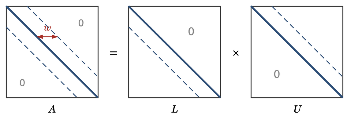
The practical gain is large. For the discretized Poisson problem, \(w=1\) and we solve the system in \(O(n)\) work, both for the factorization and for each right hand side. Had we computed \(A^{-1}\) instead, it would have been dense (as shown earlier), needing \(O(n^2)\) storage and \(O(n^2)\) work for every solve.
Two practical remarks. First, partial pivoting spoils this a little: row exchanges can widen the band of \(U\) to \(2w\). The cost stays \(O(w^2n)\) in order of magnitude, so the loss is acceptable in exchange for stability. Second, the happy \(w=1\) situation is special to one dimension. Discretizing Poisson’s equation on a two-dimensional \(N\times N\) grid gives \(n=N^2\) unknowns with half bandwidth \(w=N\), so direct elimination costs \(O(w^2n) = O(N^4) = O(n^2)\). In three dimensions it is worse still. This is precisely the point at which one abandons direct elimination and turns to iterative methods such as the conjugate gradient method; those are covered in the optimization notes.
12. Looking ahead
Two threads have been left deliberately loose.
The first is ill conditioning. Round off was blamed on the algorithm above, and partial pivoting fixed it. But some systems are hard to solve accurately no matter how good the algorithm is: a tiny perturbation of \(b\) produces a large change in \(x\). That is a property of \(A\) itself, measured by the condition number \(\kappa(A) = \|A\|\,\|A^{-1}\|\). We need matrix norms and eventually the SVD to say anything useful about it, so it is postponed.
The second is the language of vector spaces. Several times in this chapter we said things like "the columns lie in a plane", "the solution set has dimension \(n-1\)", and "there is a free variable". These are all statements about subspaces, and the next chapter is devoted to making them precise. Once that is done, the results here about existence and uniqueness will be seen as statements about four particular subspaces attached to \(A\).