Chapter 3 closed the geometry of a single matrix: lengths, angles, projections, and the four subspaces fitted together. This chapter answers a narrower question, and it answers it because the next chapter cannot start without it.
The question comes from the eigenvalue problem. We want vectors that a matrix only stretches, \(Ax = \lambda x\) with \(x \neq 0\). Rewritten, that is
so \(\lambda\) is an eigenvalue exactly when \(A - \lambda I\) is singular. Chapters 1 and 2 already give tests for singularity: eliminate and count the pivots you can finally produce, or compute the rank, or find a nonzero vector in the null space. Every one of them is a procedure you run on a matrix you already have. Here \(\lambda\) is the unknown, so what is needed instead is a single number computed from a matrix, vanishing exactly when that matrix is singular. Then \(\det(A-\lambda I) = 0\) becomes one scalar equation in \(\lambda\), and the eigenvalues are its roots.
That is what a determinant is for in this course. It is a poor way to solve a system or invert a matrix — elimination beats it at both — but it replaces "find a \(\lambda\) making this matrix singular" with a single scalar equation whose solutions are exactly the eigenvalues.
This chapter proves that equivalence and stops there. Turning \(\det(A-\lambda I)\) into an explicit polynomial in \(\lambda\) needs a formula for the determinant in terms of the entries, such as the cofactor expansion (GS §4.3); the last section says more.
Chapter 1 also wrote the \(k\)-th pivot as \(d_k = \det A_k/\det A_{k-1}\), without proof. Section 4 proves it.
1. The determinant of a \(2\times 2\) matrix, and three rules
For \(2\times 2\) there is a formula:
Throughout this chapter \(A\) is a square real matrix, \(n\times n\). For larger matrices we will not write a formula at all. Instead we ask what a determinant must do, list three rules, and derive the rest. The reason for working this way is practical: the rules are what the proofs use, and a closed formula for \(n\times n\) has \(n!\) terms and is unusable beyond \(n=3\).
Rule 1 (normalisation). \(\det I_n = 1\).
Rule 2 (row exchange). Exchanging two rows reverses the sign of the determinant.
Rule 3 (linearity in one row). With all other rows held fixed, the determinant is a linear function of the first row. That is, for scalars and vectors written out,
All three hold for the \(2\times 2\) formula, by direct computation: \(\det I = (1)(1)-(0)(0) = 1\); exchanging the rows gives \(cb - da = -(ad-bc)\); and \((a+a')d - (b+b')c = (ad-bc) + (a'd-b'c)\), while \((ta)d - (tb)c = t(ad-bc)\).
Rule 3 mentions only the first row, but Rule 2 extends it to every row: to work on row \(i\), exchange it with row 1, apply Rule 3, and exchange back. The two sign changes cancel.
1.1. Two traps in Rule 3
Rule 3 is linearity in one row at a time, with the others frozen. It is not linearity in the matrix, and the two are easy to confuse.
The determinant is not additive in the matrix. Take \(A = B = I\) of size \(2\):
Nor does a scalar come out as a single factor. Scaling the whole matrix scales every one of the \(n\) rows, so Rule 3 applies \(n\) times:
For the example above, \(\det(2I_2) = 2^2\det I_2 = 4\), which is what the arithmetic gave.
2. What the three rules force
Everything in this section follows from Rules 1 to 3 alone. The pattern of the arguments is the same throughout: produce two expressions for the same determinant, and let them contradict each other unless the determinant is zero.
Theorem 4.1. If two rows of \(A\) are equal, then \(\det A = 0\).
Proof
Exchange the two equal rows. The matrix is unchanged, so its determinant is unchanged. But Rule 2 says the exchange reverses the sign. Writing \(D\) for the determinant, \(D = -D\), hence \(2D = 0\) and \(D = 0\).
Theorem 4.2. Subtracting a multiple of one row from another leaves the determinant unchanged. That is, if \(A'\) is obtained from \(A\) by \(\text{row } i \to \text{row } i - m\,(\text{row } j)\) with \(i \neq j\), then \(\det A' = \det A\).
Proof
Apply Rule 3 to row \(i\), which is now a sum of two pieces:
In \(M\), row \(i\) is \(-m\) times row \(j\). Pull the scalar out by Rule 3 to get \(\det M = -m \det N\), where \(N\) has row \(i\) equal to row \(j\). Two rows of \(N\) are equal, so \(\det N = 0\) by Theorem 4.1, and therefore \(\det M = 0\). Hence \(\det A' = \det A\).
This is the result that makes determinants computable. Elimination is built out of exactly these operations, so it does not change the determinant at all; only the row exchanges do, and each of those reverses the sign.
Theorem 4.3. If a row of \(A\) is entirely zero, then \(\det A = 0\).
Proof
A zero row is \(0\) times itself. Pulling that scalar out by Rule 3 gives \(\det A = 0\cdot\det A = 0\).
Theorem 4.4. If \(A\) is triangular, then \(\det A = a_{11}a_{22}\cdots a_{nn}\), the product of the diagonal entries.
Proof
Take \(A\) upper triangular. The lower triangular case is the mirror image of everything below: clear below the diagonal working forwards from the first column, and in Case 2 take \(k\) to be the smallest index with \(a_{kk}=0\) and clear row \(k\) leftwards using rows \(k-1,\ldots,1\). It cannot instead be obtained from the upper triangular case by transposing, because the transpose rule, Theorem 4.7 below, is itself proved using the lower triangular case.
Case 1: every diagonal entry is nonzero. Working from the last column backwards, use row operations to clear every entry above the diagonal: to remove \(a_{ik}\) with \(i<k\), subtract \(a_{ik}/a_{kk}\) times row \(k\) from row \(i\), which is legitimate because \(a_{kk}\neq 0\). By Theorem 4.2 none of these steps changes the determinant, and they leave the diagonal matrix \(\operatorname{diag}(a_{11},\ldots,a_{nn})\). Now pull each diagonal entry out of its own row by Rule 3, \(n\) times in succession, leaving \(I\):
the last step by Rule 1.
Case 2: some diagonal entry is zero. Then the claimed product is zero, so we must show the determinant is zero too. Let \(k\) be the largest index with \(a_{kk} = 0\) — largest, because that is what makes \(a_{k+1,k+1},\ldots,a_{nn}\) all nonzero, and each of them is about to be divided by. Row \(k\) is
zero in the first \(k-1\) columns because \(A\) is upper triangular, and zero in column \(k\) by assumption. Now clear the rest of it: subtract \(a_{k,k+1}/a_{k+1,k+1}\) times row \(k+1\) to kill the entry in column \(k+1\), then the corresponding multiple of row \(k+2\), and so on to row \(n\). Each step is available because the diagonal entry it divides by is nonzero, and each leaves columns to the left untouched. After \(n-k\) steps row \(k\) is entirely zero, and by Theorem 4.2 the determinant has not changed. Theorem 4.3 now gives \(\det A = 0\).
Theorem 4.5. \(A\) is singular if and only if \(\det A = 0\). Equivalently, \(A\) is invertible if and only if \(\det A \neq 0\).
Proof
Run elimination with row exchanges as needed. Chapter 1 showed that this always ends at an upper triangular array \(U\), and that \(A\) is nonsingular exactly when it produces \(n\) nonzero pivots — the diagonal entries of \(U\). (Chapter 1’s Theorem 1.8, that the exchanges can be collected into a single \(P\) with \(PA=LU\), is stated there without proof and only for nonsingular \(A\); nothing here needs it.)
Every step of that elimination is either a row operation, which leaves the determinant alone by Theorem 4.2, or a row exchange, which flips its sign by Rule 2. So if \(r\) exchanges were used,
the second equality by Theorem 4.4. Since \((-1)^r \neq 0\), the determinant vanishes exactly when some \(u_{ii}\) is zero, which is exactly when \(A\) is singular.
This is the theorem the eigenvalue problem asked for: \(\lambda\) is an eigenvalue of \(A\) precisely when \(A - \lambda I\) is singular, which by Theorem 4.5 is precisely when \(\det(A-\lambda I) = 0\).
Equation (5) also says how a determinant is actually computed: eliminate, multiply the pivots, and fix the sign by counting exchanges. That is \(O(n^3)\) work, the same as solving a linear system.
3. Products and transposes
Theorem 4.6 (product rule). For any \(n\times n\) matrices \(A\) and \(B\), \(\det(AB) = \det A \,\det B\).
Proof
The strategy is to break \(A\) into factors whose effect on a determinant is already known: unit triangular factors change nothing, and a diagonal factor multiplies by its diagonal product.
First, two observations.
(i) Left multiplication by a unit triangular matrix changes no determinant. A unit lower triangular \(L\) is a product of elementary matrices, each adding a multiple of one row to a later row; multiplying \(M\) on the left by such a matrix performs exactly that row operation on \(M\). By Theorem 4.2 each leaves the determinant alone, so \(\det(LM) = \det M\). The same holds for unit upper triangular matrices, with the factors taken in decreasing column order. Putting \(M=I\) also gives \(\det L = 1\) for any unit triangular \(L\).
(ii) \(\det(DM) = \det D\,\det M\) for diagonal \(D\). Row \(i\) of \(DM\) is \(d_{ii}\) times row \(i\) of \(M\). Pulling out one scalar per row by Rule 3, \(n\) times,
\(\det(DM) = d_{11}\cdots d_{nn}\det M = \det D\,\det M ,\)
the last step by Theorem 4.4.
Now take \(A\) nonsingular, with \(PA = LU\) from Chapter 1. Split \(U = DU_1\) where \(D = \operatorname{diag}(u_{11},\ldots,u_{nn})\) and \(U_1\) is unit upper triangular; this is possible because every \(u_{ii}\neq 0\) when \(A\) is nonsingular. Then \(PA = LDU_1\), and
using (i), then (ii), then (i) again. The same chain with \(B = I\) gives \(\det(PA) = \det D\). Here \(P\) is the product of the \(r\) exchanges elimination made, so \(\det P = (-1)^r\) by Rule 2 — one sign change each — and \(\det(PM) = (-1)^r\det M\) for every \(M\), because left multiplication by \(P\) performs those same \(r\) exchanges on \(M\). Dividing,
If instead \(A\) is singular, then \(AB\) is singular too: each column of \(AB\) is \(A\) times a column of \(B\), so it lies in \(C(A)\), giving \(C(AB)\subseteq C(A)\) and hence \(\operatorname{rank}(AB)\leq\operatorname{rank}(A) < n\). Both sides are then zero by Theorem 4.5.
Taking \(B = A^{-1}\) gives \(\det A\,\det(A^{-1}) = \det I = 1\), so
And the product rule is what justifies the Matlab identity in the Chapter 1 companion page, where \(\det A\) is read off as \(\det(P)\prod_i u_{ii}\): that is equation (5) with the sign written as \(\det P\) instead of \((-1)^r\).
Theorem 4.7. For any square \(A\), \(\det A = \det A^T\).
Proof
Take \(A\) nonsingular first, with \(PA = LDU_1\) as in the previous proof: \(L\) unit lower triangular, \(D\) diagonal, \(U_1\) unit upper triangular. By Theorem 4.6 and Theorem 4.4,
Transposing, \((PA)^T = U_1^TD^TL^T = U_1^TDL^T\), since a diagonal matrix is its own transpose. Here \(U_1^T\) is unit lower triangular and \(L^T\) is unit upper triangular, so the same computation gives \(\det\big((PA)^T\big) = \det D\) as well. So \(\det(PA) = \det\big((PA)^T\big)\).
It remains to remove the \(P\). Now \((PA)^T = A^TP^T\), so the last equality reads \(\det P\det A = \det A^T\det P^T\). A permutation matrix satisfies \(P^TP = I\) (Chapter 1, Claim 1.7), so \(\det P^T\det P = 1\); with \(\det P = \pm 1\) this forces \(\det P^T = \det P\). Cancelling the common nonzero factor gives \(\det A = \det A^T\).
If \(A\) is singular then so is \(A^T\), because \(\operatorname{rank}A^T = \operatorname{rank}A\) (Chapter 2), and both determinants are zero by Theorem 4.5.
By Theorem 4.7, every statement about rows in this chapter has a matching statement about columns: Rules 2 and 3 were stated for rows, and transposing turns each into the corresponding rule for columns. Two equal columns give a zero determinant, a column operation changes nothing, and elimination may be run on columns instead if that happens to be easier.
4. The pivot formula of Chapter 1
Chapter 1 stated, without the means to prove it, that the \(k\)-th pivot is a ratio of determinants of leading blocks. Write \(A_k\) for the leading \(k\times k\) block of \(A\).
Theorem 4.8. Suppose \(A\) has an \(LU\) factorization with no row exchanges, with pivots \(d_1,\ldots,d_n\), all nonzero — equivalently, every leading block \(A_k\) is nonsingular (Chapter 1, Theorem 1.6). Then \(\det A_k = d_1d_2\cdots d_k\) for each \(k\), and hence
Proof
Write \(A = LU\) in block form, splitting after row and column \(k\):
where the zero blocks are forced by \(L\) being lower and \(U\) upper triangular. Multiplying, the leading block of the product is
\((LU)_k = L_kU_k + 0\cdot 0 = L_kU_k ,\)
so \(A_k = L_kU_k\). Both factors are triangular, \(L_k\) with unit diagonal and \(U_k\) with diagonal \(d_1,\ldots,d_k\). Theorems 4.6 and 4.4 give
\(\det A_k = \det L_k\,\det U_k = 1\cdot d_1d_2\cdots d_k .\)
Taking the ratio of consecutive cases gives \(d_k\), and taking \(k=n\) gives \(\det A\).
The hypothesis is needed. If elimination needs an exchange at step \(k\), the candidate \(k\)-th pivot is zero, and it is \(A_k\) — not \(A_{k-1}\) — that is singular: Chapter 1 showed \(A_k\) is nonsingular exactly when \(d_1\cdots d_{k-1}a^{(k)}_{kk}\neq 0\). The formula then still returns the right thing at step \(k\), namely \(d_k = \det A_k/\det A_{k-1} = 0\); it is the next ratio that reads \(0/0\) and says nothing. So the chain of ratios survives exactly as long as the leading blocks stay nonsingular, which is the same condition Chapter 1 gave for \(LU\) to exist without pivoting.
5. The determinant as a volume
Put the edges of a box on the rows of a matrix: the \(i\)-th row is the \(i\)-th edge vector, drawn from the origin. The claim is that \(|\det A|\) is the volume of the box those edges span — area in two dimensions, volume in three, and the natural generalisation above that. The absolute value is there because a determinant can be negative: exchanging two edges swaps the sign without changing the box, so the sign records the ordering of the edges rather than anything about their size.
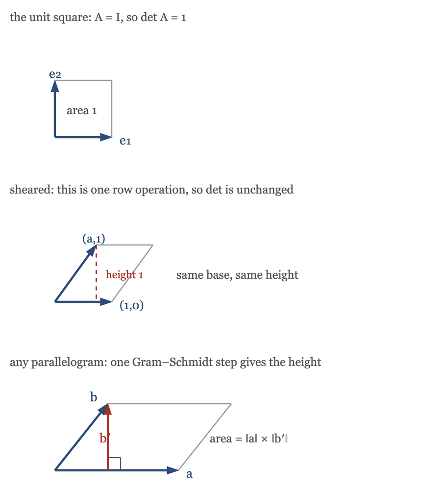
The unit square is the starting point: its edges are \(e_1\) and \(e_2\), the matrix is \(I\), and Rule 1 says the determinant is \(1\). Both agree with an area of \(1\).
Now shear it. Take edges \((1,0)\) and \((a,1)\), so
The parallelogram has the same base and the same height as the square, so the same area. The determinant agrees, and the reason it agrees is Theorem 4.2: passing from \(I\) to \(A'\) adds a multiple of one row to another, which is precisely the row operation that leaves determinants alone. Shear invariance of area and Theorem 4.2 are two statements about different quantities, and they match — which is what makes the identification of determinant with volume possible at all.
For a general parallelogram with edges \(a\) and \(b\), the same idea reduces it to a rectangle. Replace \(b\) by
which is one step of Gram—Schmidt from Chapter 3: it subtracts the component of \(b\) along \(a\) and leaves the perpendicular part, the height of the parallelogram on base \(a\). It is also a row operation, so by Theorem 4.2 the determinant is unchanged, and the area is unchanged because base and height are unchanged. The rows are now perpendicular, with lengths \(\|a\|\) and \(\|b'\|\), and the area is \(\|a\|\,\|b'\|\).
Besides the algebra, the argument so far has used two geometric facts. One is that a shear leaves area unchanged; the other is that a box with perpendicular edges has volume equal to the product of the edge lengths. In \(n\) dimensions the second is taken as the definition of volume, and the first is then a theorem about determinants rather than an assumption. Only the second is needed below.
Theorem 4.9. Let \(A\) be \(n\times n\). If its rows \(r_1,\ldots,r_n\) are mutually orthogonal with lengths \(\ell_1,\ldots,\ell_n\), then \(|\det A| = \ell_1\ell_2\cdots\ell_n\).
Proof
The \((i,j)\) entry of \(AA^T\) is \(r_i^Tr_j\), which is \(\ell_i^2\) when \(i=j\) and \(0\) otherwise. So \(AA^T = \operatorname{diag}(\ell_1^2,\ldots,\ell_n^2)\). Taking determinants and using Theorem 4.7 and then Theorem 4.6,
the last step by Theorem 4.4. Taking square roots, \(|\det A| = \ell_1\ell_2\cdots\ell_n\).
For a general matrix, run Gram—Schmidt on the rows. Every step subtracts a multiple of one row from another, so by Theorem 4.2 the determinant never changes, and the result has orthogonal rows. Theorem 4.9 then gives the volume as the product of their lengths.
Theorem 4.7 lets us say the same thing about columns, and that is the version that connects to Chapter 3 directly. For \(A\) with independent columns — which is Chapter 3’s hypothesis for \(QR\), and by Theorem 4.5 means \(A\) nonsingular here — Gram—Schmidt runs on the columns of \(A\) and produces \(A = QR\) with \(R_{jj} = \|a_j'\|\). Taking determinants, \(\det A = \det Q\,\det R\), and \(|\det Q| = 1\) because \(Q^TQ = I\) forces \((\det Q)^2 = 1\). So
the volume of the box spanned by the columns. Rows or columns, the answer is the same number — which is Theorem 4.7 again.
6. An exercise from Chapter 1
Chapter 1 discretized Poisson’s equation on a one-dimensional grid and arrived at the \(n\times n\) second-difference matrix
which is tridiagonal and symmetric. Chapter 1 asserted that its pivots are positive; here is the computation that supports it, and once the pivots are known to be nonzero, \(A = LDL^T\) applies.
Compute the pivots and the determinant of this matrix for general \(n\).
The first pivot is \(d_1 = 2\). The multiplier for row 2 is \(\ell_{21} = a_{21}/a_{11} = -1/2\). The elimination step subtracts \(\ell_{21}\) times row 1 from row 2, so the new \((2,2)\) entry is \(a_{22}\) minus \(\ell_{21}\) times the entry of row 1 in that same column, namely \(a_{12}=-1\):
Both minus signs cancel, which is why the \(1/2\) is subtracted and not added. (As a check, \(\det\begin{bmatrix} 2 & -1 \\ -1 & 2\end{bmatrix} = 3 = d_1d_2 = 2d_2\).)
The same step repeats down the diagonal. If \(d_k = (k+1)/k\), then \(\ell_{k+1,k} = a_{k+1,k}/d_k = -1/d_k = -k/(k+1)\), and with \(a_{k,k+1} = -1\) again,
which completes the induction. So \(d_k = (k+1)/k\), every pivot is positive, and
the product telescoping neatly. Note also that \(d_k \rightarrow 1\) as \(k\) grows, so the pivots never get near zero. That says elimination without row exchanges is safe here, and no more: it is a statement about the factorization, not about conditioning. This matrix is in fact increasingly ill-conditioned, with \(\kappa_2(A)\) growing like \(4(n+1)^2/\pi^2\) — about \(4\times 10^3\) at \(n=100\).
Theorem 4.8 gives the same answer by a different route, and the two agree. The leading \(k\times k\) block of \(A\) is the second-difference matrix of size \(k\), so \(\det A_k = k+1\) by the same telescoping computation, and
matching the induction. Two derivations of the same pivots are a reasonable check on both.
7. What this chapter leaves out
Strang’s Chapter 4 develops three things this chapter does not: the explicit formula for \(\det A\) as a signed sum over all \(n!\) permutations, the cofactor expansion along a row or column, and Cramer’s rule with the formula \(A^{-1} = C^T/\det A\) for the inverse.
The \(n!\) formula and Cramer’s rule are left out because this course does not compute with them: determinants are computed here by elimination, equation (5), which is what any library routine does and takes \(O(n^3)\) operations rather than \(O(n!)\). The \(n!\) formula is also one way to show that a function obeying Rules 1 to 3 exists for every \(n\); this chapter assumes that such a function exists.
The cofactor expansion is left out too. It is what shows that \(\det(A-\lambda I)\) is a polynomial in \(\lambda\), and it is how a \(3\times 3\) characteristic equation is written down by hand; GS §4.3 has it. Chapter 5 uses the polynomial fact without proof.
8. Looking ahead
The eigenvalue problem now has a usable form. By Theorem 4.5, \(\lambda\) is an eigenvalue of \(A\) exactly when
The left-hand side turns out to be a polynomial of degree \(n\) in \(\lambda\) — the characteristic polynomial — so an \(n\times n\) matrix has \(n\) eigenvalues counted with multiplicity, possibly complex. Chapter 5 states this without proof; establishing it needs a formula for the determinant in terms of the entries, such as the cofactor expansion of GS §4.3. This chapter has proved only the equivalence, which turns the search for eigenvalues into root-finding; each eigenvector is then whatever the null space of \(A-\lambda I\) turns out to contain.