EE5120 Linear Algebra - Orthogonality

A vector is a list of numbers, and there is more than one reasonable way to turn a list into a single number that measures its size. In the plane, the distance between \(A=(x_A,y_A)\) and \(B=(x_B,y_B)\) is

which is the one from school geometry. But if \(A\) is your office and \(B\) is a coffee shop three blocks away in a city laid out on a grid, that number is of no use to you: you cannot walk through buildings. What you actually walk is the sum of the horizontal and vertical distances, and that is a different measure of the same displacement. Neither is more correct than the other. They answer different questions.

So we do not fix one formula. We fix a list of properties that any sensible measure of size must have, and call anything satisfying them a norm.

Property 3 is not independent of the other two. Homogeneity with \(\alpha=0\) gives \(p(0) = 0\), and the triangle inequality applied to \(v\) and \(-v\) then gives

so \(p(v)\geq 0\) for free. It is listed anyway, because it is the property one checks first.

The standard family is

Three members of the family carry names.

The last of these needs a word, since \(\infty\) does not fit into the formula. Let \(M = \max_i|x_i|\) and suppose \(M>0\). Then

because the sum has one term equal to \(M^p\) and at most \(n\) terms each at most \(M^p\). Since \(n^{1/p}\to 1\) as \(p\to\infty\), the middle quantity is squeezed onto \(M\).

The restriction \(p\geq 1\) is needed for the triangle inequality and not for anything else. For \(p<1\) the formula still produces a number, but it fails: in \(\mathbb{R}^2\) with \(p=1/2\), take \(u=(1,0)\) and \(v=(0,1)\). Then \(\|u\|_{1/2} = \|v\|_{1/2} = 1\) while \(\|u+v\|_{1/2} = (1+1)^2 = 4\), which is not \(\leq 2\).

For the Euclidean norm we have the compact form we will use constantly. For \(x \in \mathbb{R}^n\),

and for \(x \in \mathbb{C}^n\) the same quantity is \(x^Hx = \sum_i |x_i|^2\), where \({}^H\) is the conjugate transpose introduced in Chapter 1. The conjugate is not optional: \(x^Tx\) for \(x=(1,i)\) is \(1 + i^2 = 0\), which would make a nonzero vector have zero length. From here on \(\|x\|\) with no subscript means \(\|x\|_2\).

A caution before we go on. The Euclidean norm is the natural one when the entries of \(x\) are lengths in the same units. It is a bad choice when they are not — if \(x_1\) is a voltage and \(x_2\) a temperature, then \(x_1^2 + x_2^2\) adds volts squared to kelvins squared and the answer depends on whether you measured in millivolts. It is also the wrong measure on a curved surface: the distance from Chennai to Delhi is not the straight line through the earth. Which norm to use is a modelling decision, not a mathematical one.

Only the triangle inequality is at all hard to verify for \(\|\cdot\|_2\), and it follows from an inequality that we will use far beyond that one purpose.

Theorem 3.1 (Cauchy—​Schwarz). For all \(x,y \in \mathbb{R}^n\),

with equality exactly when \(x\) and \(y\) are parallel, i.e. one is a scalar multiple of the other.

Corollary 3.2 (triangle inequality). \(\|x+y\| \leq \|x\| + \|y\|\).

So \(\|\cdot\|_2\) is a norm: homogeneity and the two zero conditions are immediate from \(\|x\|^2 = \sum_i x_i^2\), and the triangle inequality is the corollary above.

One more quantity, common in signal processing, is written like a norm and is not one:

the number of nonzero entries. For \(x = (1,0,2,2)\) we get \(\|x\|_0 = 3\). The notation comes from letting \(p\to 0\) in \(\sum_i |x_i|^p\) and using \(0^0 = 0\), \(\alpha^0 = 1\) for \(\alpha \neq 0\), so that each nonzero entry contributes \(1\) to the sum.

It fails the first axiom, and only the first. Doubling a vector does not change how many of its entries are nonzero, so \(\|2x\|_0 = \|x\|_0\), whereas homogeneity demands \(\|2x\|_0 = 2\|x\|_0\). Non-negativity is clear, \(\|x\|_0 = 0\) only for \(x=0\) is clear, and the triangle inequality does hold, since a position where \(x_i + y_i \neq 0\) must have \(x_i\neq0\) or \(y_i\neq0\). It is still an extremely useful thing to count, and it will reappear when we ask for the sparsest solution of an under-determined system.

Matrices are also vectors — the \(m \times n\) matrices form a vector space, as Chapter 2 noted — so they can be given a norm too. The simplest is to forget the shape and treat the matrix as a long list:

This is the Frobenius norm, and it is the Euclidean norm of the flattened matrix, so it is a norm for the reasons already given. It is not the only matrix norm, and it is not the one that governs how much \(A\) can stretch a vector; that one needs the singular value decomposition, and with it the condition number \(\kappa(A)\) that Chapter 1 left open. Frobenius is what one uses when the question is "how big are the entries", not "how much does \(A\) amplify".

In the plane, two vectors are perpendicular when the triangle they make obeys Pythagoras. Write that out. Vectors \(x\) and \(y\) with the third side \(x-y\) satisfy \(\|x\|^2 + \|y\|^2 = \|x-y\|^2\) exactly when

i.e. exactly when \(x^Ty=0\). So the geometric condition and the algebraic one are the same condition, and we may as well take the algebraic one as the definition, where it makes sense in every dimension.

That last remark is used constantly below. Almost every uniqueness proof ends with "this vector lies in two spaces that are perpendicular to each other, so it is perpendicular to itself, so it is zero".

The same expansion with \(x+y\) in place of \(x-y\) reads \(\|x+y\|^2 = x^Tx + 2x^Ty + y^Ty\), which equals \(\|x\|^2+\|y\|^2\) exactly when \(2x^Ty = 0\). That is the theorem in its usual form.

Theorem 3.3 (Pythagoras). \(\|x+y\|^2 = \|x\|^2 + \|y\|^2\) if and only if \(x\perp y\).

For nonzero \(x\) and \(y\), Cauchy—​Schwarz says

so there is exactly one angle \(\theta\) in the range \(0\) to \(\pi\) whose cosine is that ratio. We define the angle between \(x\) and \(y\) by

In two and three dimensions this reproduces the familiar \(\vec a \cdot \vec b = |\vec a||\vec b|\cos\theta\) of vector analysis, with \(\vec a \cdot \vec b\) written as \(a^Tb\). In \(\mathbb{R}^{50}\) there is no picture to appeal to, and the definition is all we have — which is exactly why Cauchy—​Schwarz had to be proved first. Without it, the right hand side could exceed \(1\) and the definition would be empty. Orthogonality is the case \(\theta = \pi/2\).

Independence was a rank question in Chapter 2 and needed elimination to settle. Orthogonality settles it in three lines.

Theorem 3.4. Let \(v_1,\ldots,v_k\) be nonzero and mutually orthogonal, i.e. \(v_i^Tv_j = 0\) for \(i \neq j\). Then they are linearly independent.

The hypothesis that the vectors are nonzero cannot be dropped: \(\{0\}\) alone is a mutually orthogonal set and is dependent.

Combined with part (i) of Corollary 2.5 — any \(k\) independent vectors in a \(k\)-dimensional space form a basis of it — this says that \(n\) nonzero mutually orthogonal vectors in \(\mathbb{R}^n\) are automatically a basis. Such a basis is called an orthogonal basis, and if in addition every \(\|v_i\|=1\) it is an orthonormal basis. Both conditions are captured in one line by writing

where \(\delta_{ij}\) is \(1\) for \(i=j\) and \(0\) otherwise.

The definition asks for every vector of \(V\) against every vector of \(W\). Run through the possibilities in \(\mathbb{R}^3\):

The last one needs an argument, because the picture misleads. The floor of a room and one of its walls look perpendicular, and every schoolbook says they meet at a right angle. But they share a line — the line where wall meets floor — and a nonzero vector \(u\) along that line lies in both. If the two planes were orthogonal subspaces we would need \(u^Tu = 0\), so \(u=0\). Contradiction.

The step used there is general, and we will use it again: if \(V\perp W\) then \(V\cap W = \{0\}\), because a vector lying in both is orthogonal to itself. Once we can count dimensions we will be able to rule out two planes without appealing to a room at all.

Orthogonality of two given subspaces is one thing. A more useful construction is to start with one subspace and collect everything perpendicular to it.

Two things to check straight away. First, \(V^\perp\) really is a subspace: if \(x_1,x_2\in V^\perp\) then for every \(v \in V\),

so \(\alpha x_1 + \beta x_2 \in V^\perp\). Second, \(V\perp W\) does not mean \(W = V^\perp\). Take \(V\) to be the \(x\) axis in \(\mathbb{R}^3\) and \(W\) the \(y\) axis. Every vector of \(V\) is orthogonal to every vector of \(W\), so \(V\perp W\). But \(V^\perp\) is the whole \(yz\) plane, and \(W\) is only a line inside it. Being orthogonal is a property of a pair; being the complement means being all of what is orthogonal, and \(W\) is not big enough.

Two properties of the complement will keep coming back and are recorded now.

Claim 3.5. \(V \cap V^\perp = \{0\}\), and \(V \subseteq (V^\perp)^\perp\).

The second statement is a containment, or inclusion: one space sits inside the other, with no claim yet that they coincide. It will be upgraded to equality once we can count dimensions.

Chapter 2 proved the two perpendicularity statements (Claim 2.8). With the word complement available we can say something stronger: those subspaces are not merely perpendicular, they are complete complements of each other, so that nothing perpendicular to one has been left out of the other.

Theorem 3.6. For any \(m\times n\) matrix \(A\),

Pairing Theorem 3.6 with Claim 3.5 turns the statement round, but only one way: \(C(A^T) \subseteq (C(A^T)^\perp)^\perp = N(A)^\perp\), and in the same way \(C(A)\subseteq N(A^T)^\perp\). The matching equalities need Corollary 3.8 and arrive two results from here. Note also what the theorem does to the solvability condition of Chapter 2: \(Ax=b\) is solvable iff \(b\in C(A)\), which now reads iff \(b \perp N(A^T)\). Depending on the problem, one of the two forms is easier to check than the other.

Theorem 3.7. If \(V\) is a subspace of \(\mathbb{R}^n\) with \(\dim V = r\), then \(\dim V^\perp = n-r\).

A first use of it settles the two-planes question left open above. If \(V\perp W\), then every vector of \(W\) is orthogonal to every vector of \(V\), which is exactly the statement \(W\subseteq V^\perp\). A basis of \(W\) is then an independent set sitting inside \(V^\perp\), and Chapter 2 showed that an independent set can never be larger than a spanning set, so \(\dim W \leq \dim V^\perp\). Hence

Two planes in \(\mathbb{R}^3\) would need \(2+2 \leq 3\), so no two planes in \(\mathbb{R}^3\) are orthogonal — the room argument, without the room. It also says again that \(V^\perp\) is as large as an orthogonal partner can be: \(W=V^\perp\) is the case of equality.

For the four subspaces this is just the dimension count of Chapter 2 seen again: in \(\mathbb{R}^n\) the row space has dimension \(r\) and its complement the null space has \(n-r\); in \(\mathbb{R}^m\) the column space has \(r\) and the left null space \(m-r\). Nothing new is being claimed there. What is new is that the same statement holds for any subspace, whether or not it arrived attached to a matrix.

Corollary 3.8. \((V^\perp)^\perp = V\).

This closes the pairing left half-finished after Theorem 3.6. Taking complements there, \(N(A)^\perp = (C(A^T)^\perp)^\perp\), which the corollary identifies as \(C(A^T)\); and in the same way \(N(A^T)^\perp = C(A)\). Those two equalities are what was promised at the end of Chapter 2.

Now the result that the four-subspace picture was waiting for.

Theorem 3.9. Let \(V\) be a subspace of \(\mathbb{R}^n\). Every \(x \in \mathbb{R}^n\) can be written as

and in exactly one way. Moreover \(\|x\|^2 = \|v\|^2 + \|w\|^2\).

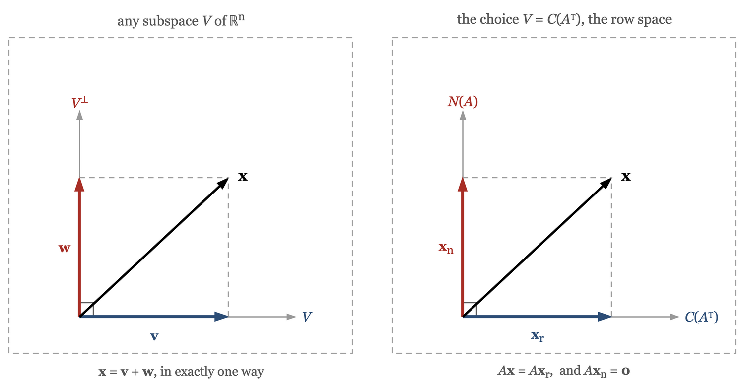
Applying this with \(V = C(A^T)\) gives the statement Chapter 2 deferred: every \(x\in\mathbb{R}^n\) splits in exactly one way as

and applying it with \(V = C(A)\) splits every \(y\in\mathbb{R}^m\) into a column space part and a left null space part. The two halves of the four-subspace figure account for the whole of each space, with no overlap and nothing left over.

Theorem 3.10. \(A\) maps the row space one-to-one and onto the column space. That is, for every \(b \in C(A)\) there is exactly one \(x_r\in C(A^T)\) with \(Ax_r = b\).

Chapter 2 proved this same statement (Claim 2.12) by a longer route, before complements were available; the proof above is the short one it promised. It also explains what a pseudo-inverse \(A^{ + }\) can and cannot do. Restricted to the row space, \(A\) is invertible, so there is a sensible map sending \(b=Ax_r\) back to \(x_r\), and \(A^{ + }(Ax_r) = x_r\). But \(A\) sends the whole null space to the single vector \(0\), and no map can undo that: \(A^{ + }(Ax_n) = A^{ + }0 = 0\). So \(A^{ + }A\) is not the identity in general — it is the operation "throw away \(x_n\), keep \(x_r\)", which is a projection. Only when \(r=m=n\) do the null space and left null space both collapse to \(\{0\}\) and \(A^{ + }\) become a genuine inverse.

Here is the situation that makes this section necessary, in the form it usually arrives.

A satellite such as NISAR looks down at the earth with a radar and records the backscattered power \(\sigma\) from each patch of ground. What you actually want to know is not \(\sigma\) but the soil moisture, the vegetation water content, the tree cover — call them \(x_1,\ldots,x_n\). You propose a linear model,

and you go to a test site where the \(x_i\) have been measured on the ground, so that each visit gives you one equation in the \(n+1\) unknown coefficients \(\beta_0,\ldots,\beta_n\). Collect \(n+1\) visits and you have a square system \(A\beta = \sigma\), which you solve if \(A\) is invertible.

That is the textbook answer and it is a bad plan. The radar readings carry noise, the ground measurements carry noise, and the linear model itself is an approximation. Solving a square system forces the model to pass exactly through \(n+1\) noisy points, and the coefficients you get will lurch around when you repeat the exercise at a different site. What you want instead is to visit many more than \(n+1\) sites, so that the errors have a chance to average out, and then ask for the coefficients that fit all of them as well as possible.

A smaller version of the same thing, which we will carry through the section. A craft starts at time \(t=0\) with unknown initial velocity \(u\) and constant unknown acceleration \(a\), so its velocity obeys

Measure \(v\) at times \(t_1,t_2,\ldots,t_m\) and you get

Two measurements suffice if there is no noise. With noise you take \(m \gg 2\), and \(A\) is a tall matrix, \(m > n\). Note that the model is linear in the unknowns \(u\) and \(a\), which is all that is required; it is not linear in \(t\), and it need not be. Fitting \(v = u + at + bt^2\) or \(v = u + at + b\ln t\) is the same kind of problem with a different third column.

We assume throughout this section that the columns of \(A\) are independent. For the velocity problem that says the \(t_i\) are not all equal, which is a statement about the experiment being sensible: if you take all your readings at the same instant you cannot expect to learn the acceleration.

With \(m>n\) and independent columns, Chapter 2 says \(Ax=b\) has at most one solution, and has one exactly when \(b \in C(A)\). But \(C(A)\) is an \(n\)-dimensional subspace sitting inside \(\mathbb{R}^m\), and a noisy \(b\) will miss it. So generically there is no solution at all, and the honest response is not to force one but to change the question.

Define the error or residual

and look for the \(x\) that makes it as small as possible:

Measuring \(e\) in the Euclidean norm is what makes this the least squares problem — we are minimising \(\sum_j e_j^2\), a sum of squares. Other norms give other, perfectly respectable problems; \(\ell_2\) is chosen partly because it is the one that yields to linear algebra, and partly because it is the right thing to do when the noise is Gaussian, which is a story for a statistics course.

As \(x\) runs over \(\mathbb{R}^n\), the vector \(Ax\) runs over the whole of \(C(A)\) and nothing else. So the problem is really geometric, and has nothing to do with \(x\):

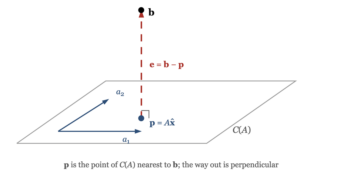
The picture says the shortest distance from a point to a plane is along the perpendicular, so \(e\) should come out perpendicular to \(C(A)\). Let us take that as a guess, derive the equations from it, and then prove that the answer really is the minimiser rather than merely a plausible candidate.

(a) Through the left null space. If \(e \perp C(A)\) then \(e \in C(A)^\perp = N(A^T)\), which by definition means \(A^Te = 0\). Substituting \(e = b - A\hat{x}\):

(b) Column by column. The column space is spanned by the columns \(a_1,\ldots,a_n\) of \(A\), and a vector orthogonal to each of them is orthogonal to every combination of them. So the condition is \(a_i^Te = 0\) for \(i=1,\ldots,n\). Stacking these \(n\) scalar equations one below the other is exactly \(A^Te = 0\), since the \(i\)th row of \(A^T\) is \(a_i^T\). Same conclusion.

(c) Through calculus, with no geometry at all. Write \(f(x) = \|b-Ax\|^2\) out in coordinates,

and set each partial derivative to zero. Differentiating with respect to \(x_i\), only the terms with \(k=i\) contribute to the inner derivative, and that inner derivative is \(-A_{ji}\):

The last sum is the \(i\)th entry of \(A^T(b-Ax)\). Setting all \(n\) of them to zero gives \(A^T(b - A\hat{x}) = 0\) again.

Everything now depends on the \(n\times n\) matrix \(A^TA\), so we collect what is known about it. Two facts are from Chapter 1 and Chapter 2; the middle one is new.

Symmetric. \((A^TA)^T = A^T(A^T)^T = A^TA\).

Same null space as \(A\). This holds for every \(A\), with no rank assumption.

Theorem 3.11. \(N(A^TA) = N(A)\) for any \(m\times n\) matrix \(A\).

The second half turns on \(x^TA^TAx\) being \(\|Ax\|^2\), a sum of squares, which vanishes only when every term does. Read as a bare scalar equation it would tell us nothing.

Invertible when the columns of \(A\) are independent. Chapter 2 proved this directly while constructing the left inverse (Theorem 2.11). It also drops out of the theorem above: independent columns mean \(N(A)=\{0\}\), hence \(N(A^TA) = \{0\}\), and by rank—​nullity applied to the square matrix \(A^TA\) we get \(\operatorname{rank}(A^TA) = n\), i.e. full rank, i.e. invertible.

Here is the same fact without the algebra. Independent columns say \(A\) loses nothing: it maps \(\mathbb{R}^n\) one-to-one into \(C(A)\). And \(A^T\) maps \(C(A)\) one-to-one back onto the row space, which here is all of \(\mathbb{R}^n\). So \(A^TA\) is a one-to-one map of \(\mathbb{R}^n\) to itself, which is what invertible means.

Theorem 3.12. Let \(A\) be \(m\times n\) with independent columns. Then the normal equations have the unique solution

and \(\hat{x}\) is the unique minimiser of \(\|b-Ax\|\). The nearest point in the column space is

Two remarks, which are often run together and should not be.

This settles the caution box of Chapter 2. The formula \((A^TA)^{-1}A^Tb\) produces an answer for every \(b\); when \(b\in C(A)\) that answer is the exact solution of \(Ax=b\), and when \(b\notin C(A)\) it is the least squares solution. Chapter 2 had no way to say what the formula computed in that second case; now we can.

Take three measurements of the craft: at \(t=-1,\,1,\,2\) the recorded velocities are \(v = 1,\,1,\,3\). Fitting \(v = x_1 + x_2 t\),

Is \(b\in C(A)\)? Three points lie on a straight line \(v = x_1+x_2t\) only if they are collinear; the first two give slope \((1-1)/(1-(-1)) = 0\) and the last two give \((3-1)/(2-1) = 2\). They are not, so \(b\notin C(A)\) and there is no exact solution. Build the normal equations, showing each entry:

The determinant is \((3)(6) - (2)(2) = 18-4 = 14\), so

Check it in the normal equations: \(3(9/7) + 2(4/7) = 27/7+8/7 = 35/7 = 5\) and \(2(9/7) + 6(4/7) = 18/7+24/7 = 42/7 = 6\). So the best straight line is \(v = 9/7 + (4/7)t\). The projection is

and the error is

Two checks, both of which should be done every time. First, \(e\) is perpendicular to both columns of \(A\):

Second, the size of what we could not fit:

The same numbers can be drawn in two entirely different pictures, and the two get confused constantly.

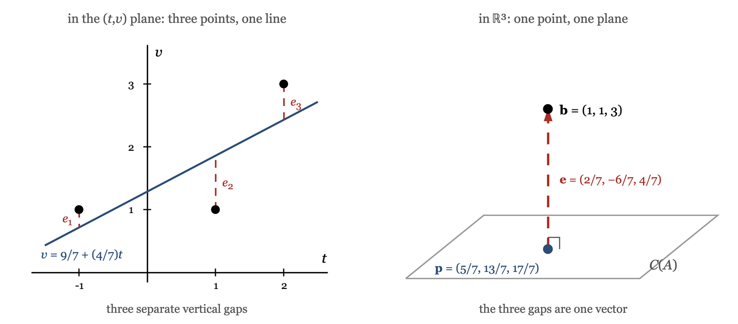
In the left picture the three errors \(e_1,e_2,e_3\) are three separate vertical gaps in a plane. In the right picture they are the three components of one vector \(e\) in \(\mathbb{R}^3\). The quantity being minimised, \(e_1^2+e_2^2+e_3^2\), is the sum of the squared gaps on the left and the squared length of a single vector on the right. Confusing the two is easy, and it is where people get lost.

Suppose you do all this and the residual \(\|e\|\) comes out unacceptably large. The least squares machinery has done its job — it found the best fit available — so the fault is elsewhere, and there are three places to look.

Not all measurements deserve equal trust. If the third reading came from an instrument you know to be poor, it should not be allowed to pull the fit as hard as the others. Give each row a weight \(w_j>0\) and minimise

This is ordinary least squares for the matrix \(WA\) and right hand side \(Wb\), so the normal equations become

Setting all \(w_j=1\) recovers the unweighted case. In practice \(w_j\) is taken as \(1/\sigma_j^2\), the reciprocal of the variance of measurement \(j\), so that a reading with twice the standard deviation counts a quarter as much. (GS section 3.3 treats this as optional reading.)

The least squares calculation produced, as a by-product, a formula that takes any \(b\) and returns the nearest point of \(C(A)\):

\(P\) is \(m\times m\) and is called the projection matrix onto \(C(A)\). The middle factor \((A^TA)^{-1}\) does not split as \(A^{-1}(A^T)^{-1}\), since for a rectangular \(A\) neither of those exists. The formula does simplify when \(A\) is square and invertible, and there it collapses to \(P=I\): such an \(A\) has \(C(A) = \mathbb{R}^m\), so every \(b\) is already in the subspace and is its own nearest point.

Two properties characterise projections.

Theorem 3.13. Let \(A\) have independent columns and \(P = A(A^TA)^{-1}A^T\). Then \(P^2 = P\) and \(P^T = P\).

The complementary projection. If \(P\) projects onto \(C(A)\), then \(I-P\) projects onto \(C(A)^\perp = N(A^T)\). Indeed \((I-P)b = b - p = e\), which we already know lies in \(N(A^T)\); and \((I-P)^2 = I - 2P + P^2 = I-P\), \((I-P)^T = I-P\). So the splitting theorem, Theorem 3.9, applied to \(b = p + e\), is implemented by the pair of matrices \(P\) and \(I-P\), which sum to \(I\).

A projection matrix is never invertible unless it is \(I\). From \(P^2=P\) we get \(P(P-I) = 0\), so every column of \(P-I\) lies in \(N(P)\); if \(P\neq I\) that null space is nonzero. Geometrically, everything in \(C(A)^\perp\) is flattened to zero and cannot be recovered.

Take the smallest case, \(n=1\): \(A\) is a single column \(a\), and \(C(A)\) is the line through the origin in the direction of \(a\). The formula still applies, with \(a^Ta\) now a single number, so it can be moved around freely:

Read the second form carefully: \(a^Tb\) is a scalar, so \(p\) is a multiple of \(a\), as it must be. And \(aa^T\) is the outer product of Chapter 1 — an \(m\times m\) matrix of rank one, every column a multiple of \(a\).

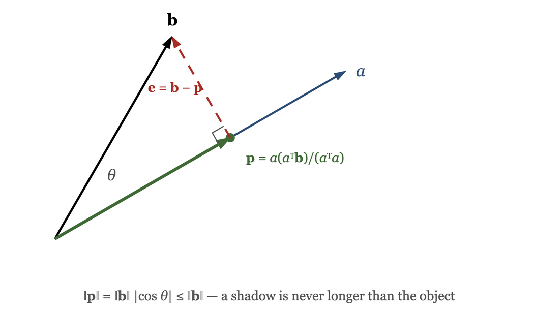
Check the perpendicularity directly, which is a one-line calculation and a good sanity test of the formula:

The line case gives a second proof of Cauchy—​Schwarz, and this one comes with a picture. Compute the length of the projection:

so \(\|p\| = |a^Tb| / \|a\|\). Now use the geometry: \(b = p + e\) with \(p\perp e\), so Pythagoras gives \(\|b\|^2 = \|p\|^2 + \|e\|^2 \geq \|p\|^2\). A shadow is never longer than the thing casting it. Therefore

which is Cauchy—​Schwarz. Equality needs \(\|e\|=0\), i.e. \(b=p\) is already on the line — the parallel case, as before.

This is the same inequality as before, now with a picture behind it. The algebraic proof came first, in the norms section, only because the triangle inequality was needed there and projections were not yet available. With the angle definition \(\cos\theta = a^Tb/(\|a\|\|b\|)\) in hand, the projection length reads

which is the school formula for the length of a shadow.

Turn the shape of the matrix round. Let \(A\) be \(m\times n\) with \(m<n\) — a fat matrix, fewer measurements than unknowns — and assume its rows are independent, i.e. \(r=m\). The four subspaces then have dimensions

Since \(\dim C(A) = m\) and \(C(A)\subseteq\mathbb{R}^m\), the column space is all of \(\mathbb{R}^m\). So \(Ax=b\) is solvable for every \(b\), noise or no noise, and the minimum error is exactly zero. Least squares has nothing to offer here; there is no error to minimise.

The difficulty is the opposite one. There are \(n-m>0\) free variables, so the solution set is \(x_p + N(A)\), an infinite family. Which member of it should we report?

A natural criterion, and the one that turns out to be tractable, is to ask for the shortest solution — in an electrical setting, the one of least energy:

Theorem 3.9 answers it immediately. Write any solution as \(x = x_r + x_n\) with \(x_r \in C(A^T)\) and \(x_n\in N(A)\). Then \(Ax = Ax_r + Ax_n = Ax_r\), so the null space part contributes nothing to satisfying the equation; but by Pythagoras it does contribute to the length,

So the shortest solution is the one with \(x_n=0\): the solution lying in the row space. And the row space part is the same for every solution, since two solutions differ by a null space vector. There is therefore exactly one shortest solution, and it is \(x_r\).

Theorem 3.14. If \(A\) is \(m\times n\) with independent rows, then \(AA^T\) is invertible and the minimum norm solution of \(Ax=b\) is

The matrix \(C = A^T(AA^T)^{-1}\) is exactly the right inverse built in Chapter 2, and \(AC = AA^T(AA^T)^{-1} = I_m\) as it should. Chapter 2 remarked that the right inverse is not unique when \(m<n\) (Theorem 2.10); we can now say what is special about this particular one. It is the choice that lands in the row space, and therefore the choice that returns the shortest answer.

The two cases are dual, and are easy to mix up, so here they are side by side.

One sentence covers both formulas: \(A^{ + }b\) is the row space vector that \(A\) maps to the nearest reachable point to \(b\). In the tall case "nearest" does the work; in the fat case "row space" does. The construction that handles both at once, along with the rank-deficient cases where neither \(A^TA\) nor \(AA^T\) is invertible, is the singular value decomposition.

Minimising \(\|x\|_2\) was a choice, made because it is the one linear algebra can solve in closed form. It is not the only sensible one. Replace it by the \(\ell_1\) norm:

This has no formula, and needs the machinery of convex optimisation, but the answer it gives is qualitatively different: it tends to be sparse, with many entries exactly zero, whereas the \(\ell_2\) answer spreads itself over all \(n\) entries. What one would really like is to minimise \(\|x\|_0\), the number of nonzeros, and that problem is combinatorially hard; under conditions on \(A\) the \(\ell_1\) answer coincides with the \(\ell_0\) answer, which is the basis of the field of compressive sensing. This is where much of modern signal processing lives, and it makes a good course project.

An orthonormal basis reduces the three operations this chapter keeps needing — inverting, taking coordinates, projecting — to inner products. Collect \(n\) orthonormal vectors \(q_1,\ldots,q_n\in\mathbb{R}^n\) as columns:

Then the \((i,j)\) entry of \(Q^TQ\) is row \(i\) of \(Q^T\) times column \(j\) of \(Q\), which is \(q_i^Tq_j = \delta_{ij}\). That is the identity, entry by entry:

Inverting \(Q\) costs nothing at all — you transpose it. This is why one goes to the trouble of constructing orthonormal bases.

We have met three families of them already, without the name.

Projections, by contrast, are not orthogonal matrices, despite being built out of orthogonality. A projection matrix satisfies \(P^T=P\) and \(P^2=P\); an orthogonal matrix satisfies \(Q^TQ=I\). The only matrix doing both is \(I\) itself.

Theorem 3.15. If \(Q\) is orthogonal then \(\|Qx\| = \|x\|\) for every \(x\), and \((Qx)^T(Qy) = x^Ty\) for every \(x,y\).

Since both the inner product and the two lengths are unchanged, so is \(\cos\theta = x^Ty/(\|x\|\|y\|)\). An orthogonal matrix moves the whole space rigidly: no stretching, no shearing, no change of angle. Rotations and reflections are exactly what that description suggests.

This has a consequence for computation. Chapter 1 blamed round-off trouble on small pivots, which forced a division by a small number and amplified whatever error was already present. An orthogonal matrix cannot amplify anything: whatever error \(\delta\) is present in \(x\), the error in \(Qx\) is \(Q\delta\), of exactly the same size. An algorithm built out of orthogonal matrices does not manufacture round-off error, and that is why numerical linear algebra reaches for them at every opportunity.

The contrast with a projection is instructive. \(\|Pb\| \leq \|b\|\) always, with strict inequality unless \(b\) is already in the subspace — a projection loses length, permanently, and the lost part cannot be recovered.

Given any basis, finding the coordinates of a vector means solving a linear system. With an orthonormal basis it means taking inner products.

Let \(\{q_1,\ldots,q_n\}\) be an orthonormal basis of \(\mathbb{R}^n\) and let \(b\) be any vector. Then \(b = \sum_i x_iq_i = Qx\) for some coordinate column \(x\). To find \(x_j\), hit both sides with \(q_j^T\):

since every term but \(i=j\) dies. So \(x = Q^Tb\) — which is also what \(Qx=b\) gives when you multiply by \(Q^{-1}=Q^T\), as it must be. Written out,

The second form identifies each term as a projection: \(q_iq_i^T\) is the rank-one projection matrix onto the line through \(q_i\), since \(q_i^Tq_i=1\) makes the denominator disappear. So a vector is the sum of its projections onto the axes of an orthonormal basis, and the \(n\) rank-one matrices \(q_iq_i^T\) add up to \(I\). In the standard basis of \(\mathbb{R}^3\) this is the familiar statement that \(v = 3\hat{x} + 4\hat{y} + 5\hat{z}\) with the coefficients read off directly. In a general basis it would not be.

Lengths come along too.

Theorem 3.16 (Parseval). \(\displaystyle \|b\|^2 = \sum_{i=1}^n (q_i^Tb)^2\).

For \(v=3\hat x+4\hat y+5\hat z\) this is \(\|v\|^2 = 9+16+25\). The content of the theorem is that it holds in every orthonormal basis, not only the standard one. When the basis is a set of sines and cosines the same statement is the energy theorem of Fourier analysis, which we come to at the end of the chapter.

Claim 3.17. If a square \(Q\) has orthonormal columns then it has orthonormal rows.

The proof leans entirely on \(Q\) being square, since that is what makes a one-sided inverse two-sided. The next subsection shows that the claim is false without it.

Can \(Q\) be rectangular? Ask the definition. If \(Q\) is \(m\times n\) with \(m<n\), it has more columns than the dimension of the space they live in, so the columns must be dependent — and dependent vectors are certainly not orthonormal. A fat \(Q\) is impossible.

A tall \(Q\), \(m>n\), is perfectly possible: \(n\) orthonormal vectors in \(\mathbb{R}^m\) with \(n<m\) is no contradiction. The computation \((Q^TQ)_{ij} = q_i^Tq_j = \delta_{ij}\) goes through unchanged, so

The second cannot hold, because \(QQ^T\) has rank at most \(n<m\). So a tall \(Q\) has \(Q^T\) as a left inverse and no right inverse — consistent with Chapter 2, since a tall matrix with independent columns has exactly that. Its rows are not orthonormal: there are \(m\) of them living in \(\mathbb{R}^n\), so they are dependent.

Now feed a tall \(Q\) into the least squares machinery. With \(A=Q\), the matrix \(A^TA = Q^TQ = I\), and everything collapses:

No inverse to compute, no system to solve — the least squares solution is \(n\) inner products. It pays for the trouble of getting hold of an orthonormal basis of \(C(A)\) in the first place, and constructing one is the next section. Note that \(QQ^T\) is a projection and not the identity, which is the whole point: it is the projection onto the \(n\)-dimensional subspace \(C(Q)\) inside \(\mathbb{R}^m\), and it agrees with \(\sum_i q_iq_i^T\), the sum of the projections onto the \(n\) axes we do have.

We are given a basis \(a_1,\ldots,a_n\) of some subspace — independent, but at arbitrary angles to each other and of arbitrary lengths — and we want an orthonormal basis of the same subspace. Gram—​Schmidt does it one vector at a time, and the rule is always the same: take the next given vector, subtract off its components along everything already built, and normalise what is left.

With three vectors \(a_1,a_2,a_3\):

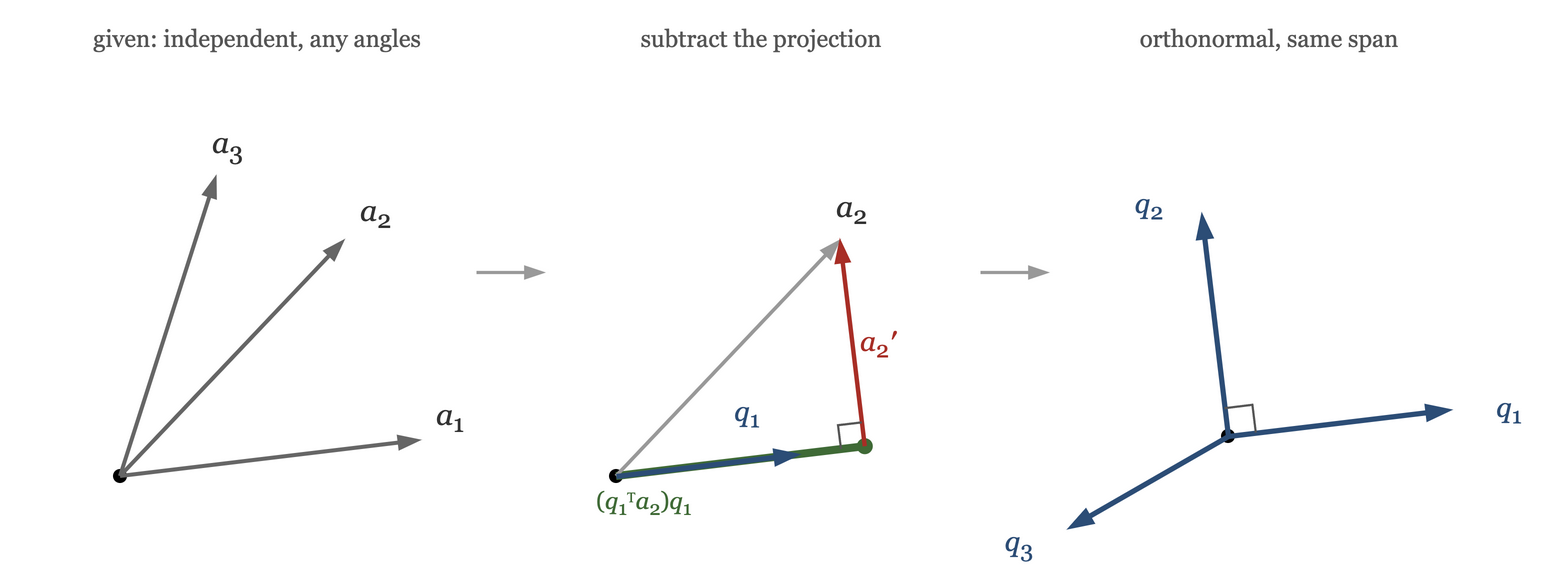
In general, at stage \(j\) there are \(j-1\) projections to subtract:

Note that \(\sum_{i<j}(q_i^Ta_j)q_i\) is exactly the projection of \(a_j\) onto the span of \(q_1,\ldots,q_{j-1}\), by the coordinate formula of the previous section. So the step is "subtract the projection onto what you have so far", which is why the leftover is perpendicular to all of it.

Theorem 3.18. If \(a_1,\ldots,a_n\) are independent, then Gram—​Schmidt never divides by zero, and the resulting \(q_1,\ldots,q_n\) are orthonormal with

The proof also gives a test for free: if at some stage \(a_k'\) comes out to be zero, the input vectors were not independent, and \(a_k\) is a combination of the earlier ones. Gram—​Schmidt detects dependence rather than silently producing nonsense.

One thing it does not give is uniqueness. Feed in the same vectors in a different order and you get a different orthonormal basis of the same space — \(q_1\) is always a multiple of whichever vector you handed over first.

Take the columns of

Step 1. \(\|a_1\|^2 = 1^2+0^2+1^2 = 2\), so

Step 2. With \(a_2 = (1,0,0)^T\), \(q_1^Ta_2 = \big((1)(1) + (0)(0) + (1)(0)\big)/\sqrt2 = 1/\sqrt2\), so

Its length is \(\sqrt{1/4 + 0 + 1/4} = 1/\sqrt2\), so

Step 3. Two inner products, with \(a_3 = (2,1,0)^T\):

So

which already has length \(1\), so \(q_3 = (0,1,0)^T\). Collecting,

Check \(Q^TQ=I\) on one entry: \(q_1^Tq_2 = \frac{1}{2}\big((1)(1) + (0)(0) + (1)(-1)\big) = 0\).

Gram—​Schmidt does not throw away information; the numbers \(q_i^Ta_j\) it computes along the way record exactly how to get the original vectors back. Since \(q_1,\ldots,q_n\) is an orthonormal basis of the space the \(a_j\) live in, the coordinate formula of the previous section says

But most of those coefficients are zero. By the span property, \(a_j\in\operatorname{span}(q_1,\ldots,q_j)\), so \(a_j\) has no component along \(q_i\) for \(i>j\), i.e. \(q_i^Ta_j=0\) whenever \(i>j\). So the sum stops at \(i=j\), and stacking the \(a_j\) as columns gives

that is, \(A = QR\) with \(R\) upper triangular and \(R_{ij} = q_i^Ta_j\).

The diagonal entries are positive, so \(R\) is invertible. From the process, \(a_j = a_j' + \sum_{i<j}(q_i^Ta_j)q_i\) with \(a_j'\perp q_i\) for \(i<j\), so

A triangular matrix with no zero on the diagonal is invertible (Lemma 1.4) — so \(R^{-1}\) exists. For an \(m\times n\) matrix \(A\) with \(m\geq n\) and independent columns, the shapes are \(A: m\times n\), \(Q: m\times n\) with orthonormal columns, \(R: n\times n\) upper triangular and invertible.

For the example above, \(R_{11} = \|a_1\| = \sqrt2\), \(R_{12} = q_1^Ta_2 = 1/\sqrt2\), \(R_{13} = q_1^Ta_3 = \sqrt2\), \(R_{22} = q_2^Ta_2\), which is \(\frac{1}{\sqrt2}\big((1)(1)(0)(0)(-1)(0)\big) = 1/\sqrt2\), then \(R_{23} = q_2^Ta_3 = \sqrt2\) and \(R_{33} = q_3^Ta_3 = (0)(2)(1)(1)(0)(0) = 1\). So

Multiply out the first column to check: \(\sqrt2\,q_1 = (1,0,1)^T = a_1\). And the third:

Substituting \(A=QR\) into the normal equations makes \(A^TA\) disappear:

and since \(R^T\) is invertible it can be cancelled from both sides, leaving

\(R\) is upper triangular, so this is solved by back substitution at a cost of about \(n^2/2\) operations — the same back substitution as in Chapter 1.

The point is not the arithmetic saving. It is that \(A^TA\) is never formed. Forming it squares the sensitivity of the problem: the condition number of \(A^TA\) is the square of that of \(A\), so a matrix that was awkward becomes hopeless. The \(QR\) route works with \(A\) itself and with orthogonal matrices, which as we saw amplify nothing. This is what library least squares solvers actually do.

Nothing is free. At stage \(j\), Gram—​Schmidt computes \(j-1\) inner products \(q_i^Ta_j\) and subtracts \(j-1\) scaled vectors, each of these being \(m\) multiply—​add pairs. So stage \(j\) costs about \(2m(j-1)\) operations, and the total is

multiply—​subtract pairs, counting as Chapter 1 did. For a square matrix, \(m=n\) and this is \(n^3\), against \(n^3/3\) for plain elimination: same order, three times the work. That is the price of orthogonality, and for an ill-conditioned problem you pay it gladly.

Two practical remarks. The version written above is classical Gram—​Schmidt, and it is the one to learn but not the one to use: in floating point the later \(q_j\) lose orthogonality badly, because each is computed from the original \(a_j\) and inherits all the accumulated error. Modified Gram—​Schmidt subtracts the projections one at a time from a running vector rather than all at once from \(a_j\), which is the same thing in exact arithmetic and much better behaved in floating point. Library routines usually do neither, and build \(Q\) as a product of reflection matrices \(I-2ww^T\) instead — Householder’s method, which is more stable still.

Two kinds of argument have been used in this chapter, and they behave differently when the dimension grows. The inner product arguments — Cauchy—​Schwarz, the triangle inequality, Pythagoras, the definition of orthogonality, Gram—​Schmidt on a finite list — rest on the algebra of \(x^Ty\) and on the single fact that \(v^Tv=0\) forces \(v=0\); the size of \(n\) never entered. The dimension counting is another matter: \(\dim V + \dim V^\perp = n\), and the splitting of \(\mathbb{R}^n\) that rests on it, used finiteness in an essential way. With that distinction in hand, let \(n\to\infty\) and ask what \(\mathbb{R}^\infty\) looks like — vectors with infinitely many entries, \(v = (v_1,v_2,v_3,\ldots)\).

Addition and scalar multiplication cause no trouble. Length does. The natural definition \(\|v\|^2 = \sum_{i=1}^\infty v_i^2\) is a sum that need not converge: for \(v = (1,1,1,\ldots)\) it is \(+\infty\), and a vector of infinite length is of no use to anybody. The repair is to admit only those vectors for which the sum is finite.

So \((1,1,1,\ldots)\) is excluded, while \(w = (1,\tfrac12,\tfrac14,\tfrac18,\ldots)\) is admitted, with

The first group of results now carries over word for word, since nothing in their proofs mentioned \(n\). The dimension-counting group does not, and repairing it is the business of a course in analysis: an infinite orthonormal set can fail to span, infinite sums have to be shown to converge, and \((V^\perp)^\perp = V\) needs \(V\) to be closed. None of that is needed below, because every subspace we project onto in this section is spanned by finitely many functions.

Now the step that makes this useful. Take a function \(f\) on an interval, say \(\sin x\) on \(0\leq x\leq 2\pi\), and chop the interval into \(N\) pieces of width \(\Delta x\). The list of sampled values

is an ordinary vector, and as \(\Delta x \to 0\) it becomes a vector with a continuum of entries — one for each \(x\). The sums that defined length and inner product become integrals:

For complex-valued functions the first factor is conjugated, \((f,g) = \int \overline{f}g\,dx\), for the same reason the conjugate appeared in \(x^Hx\). Two conditions have to be stated with the space, and both are easy to forget:

With those in place, \((f,g)\) is an inner product, \(\|f\|\) is a norm, and two functions are orthogonal when \((f,g)=0\). The first example is the one that started Fourier analysis:

They are orthogonal but not orthonormal, since \(\int_0^{2\pi}\sin^2x\,dx = \int_0^{2\pi}\frac{1-\cos 2x}{2}dx = \pi\) and likewise for \(\cos^2\). Dividing by \(\sqrt\pi\) fixes that: \(\sin x/\sqrt\pi\) and \(\cos x/\sqrt\pi\) are orthonormal over \(0\leq x\leq 2\pi\).

The claim is that the whole family

is mutually orthogonal over \(0\leq x\leq 2\pi\). The verification is three integrals, done with the product-to-sum identities. For integers \(m,n\geq 1\) with \(m\neq n\),

because \(\int_0^{2\pi}\cos kx\,dx = 0\) for every nonzero integer \(k\). The same identity gives \(\int_0^{2\pi}\sin mx\sin nx\,dx = 0\) for \(m\neq n\), and \(\int_0^{2\pi}\sin mx\cos nx\,dx = 0\) for all \(m,n\), including \(m=n\). The diagonal terms are

So this is an orthogonal basis — unnormalised, with the constant function carrying a different norm from the rest, which is the source of the stray factors of \(2\) in every Fourier series formula ever written.

Now the Fourier series itself is nothing but the coordinate formula of an orthogonal basis. Writing

and taking the inner product of both sides with \(\cos nx\), every term on the right dies except one:

Compare this with the projection of a vector \(b\) onto a line through \(a\):

It is the same formula with the same meaning. A Fourier coefficient is a projection. The series expresses \(f\) as the sum of its projections onto the axes of an orthogonal basis, exactly as \(b = \sum_i (q_i^Tb)q_i\) did in \(\mathbb{R}^n\).

There is a least squares statement hiding here too, and it is the practically important one, since one never sums infinitely many terms.

Theorem 3.19. Among all combinations of \(\{1,\cos x,\sin x,\ldots,\cos Nx,\sin Nx\}\), the one closest to \(f\) in the \(\|\cdot\|\) of this space is the truncated Fourier series, i.e. the one whose coefficients are given by the formula above.

In the matrix language of the least squares section: think of \(Mz = s\) where the columns of \(M\) are the basis functions and \(s\) is \(f\). Generally \(f\notin C(M)\) — a finite trigonometric sum cannot reproduce an arbitrary function — and the condition for the best \(p\) was that each column be orthogonal to the residual, \(m_i^T(s-p)=0\). That is exactly the line \((\cos nx, f-p)=0\) above.

Parseval’s theorem also survives the translation. In an orthonormal basis \(\|b\|^2 = \sum_i (q_i^Tb)^2\); here it reads

the unequal factors being the squared norms of the unnormalised basis functions. This is the statement that the energy of a signal can be counted in the time domain or in the frequency domain, and comes out the same.

Sines and cosines are the right basis for a periodic function. For a non-periodic one on a finite interval, a natural choice is polynomials: they are cheap to evaluate, cheap to differentiate and integrate, and if the approximation error is small there is no reason to carry the original function around. This is the premise of the finite element method and of a good deal of numerical analysis.

So take the interval \((0,1)\), the basis \(\{1,\,z,\,z^2\}\), and a given \(f\). We want coefficients with

in the least squares sense. Take the inner product of both sides with each basis function in turn — this is route (b) of the least squares section, "each column orthogonal to the residual" — and you get a \(3\times3\) system, the normal equations for this problem:

The matrix on the left is the analogue of \(A^TA\) and is called the Gram matrix of the basis. Its entries are trivial to compute here, since

giving

This is the Hilbert matrix, and it is the standard example of a matrix that is fine in theory and hopeless in practice. Run one step of elimination on it, showing the arithmetic. The multipliers are \(\ell_{21} = (1/2)/1 = 1/2\) and \(\ell_{31} = (1/3)/1 = 1/3\), so

The next multiplier is \(\ell_{32} = (1/12)/(1/12) = 1\), and the last entry becomes \(\tfrac4{45} - \tfrac1{12} = \tfrac{16}{180} - \tfrac{15}{180} = \tfrac1{180}\). The three pivots are

shrinking by more than a factor of ten each time, and this is only the \(3\times3\) case. For the \(n\times n\) Hilbert matrix the condition number multiplies by roughly \(e^{3.5}\approx 30\) for each extra row: at \(n=10\) it is about \(1.6\times10^{13}\), so about thirteen of the sixteen digits of double precision are lost, and by \(n=12\) it is around \(10^{16}\) and there is nothing left. A basis that looks entirely reasonable produces a system that cannot be solved on a computer past about ten terms.

The trouble is not the polynomials but the basis: \(z^9\) and \(z^{10}\) look nearly identical on \((0,1)\), so the basis vectors are at very small angles to one another, and the Gram matrix is nearly singular. Orthogonalise the basis and the Gram matrix becomes \(I\).

Run the process of the previous section, with inner products now meaning integrals over \((0,1)\).

Step 1. There is nothing to subtract, so \(q_0'(z) = 1\), and \(\|q_0'\|^2 = \int_0^1 1\,dz = 1\) already, giving \(q_0(z) = 1\).

Step 2. \((q_0, z) = \int_0^1 z\,dz = 1/2\), so

so \(q_1(z) = \sqrt{12}\left(z-\tfrac12\right) = 2\sqrt3\left(z - \tfrac12\right)\).

Step 3. Two projections to subtract. First \((q_0, z^2) = \int_0^1 z^2 dz = 1/3\). Second,

so that

Therefore

whose squared norm works out to \(\|q_2'\|^2 = 1/180\), giving

These are the Legendre polynomials for the interval \((0,1)\) — the shifted Legendre polynomials — and the same construction on \((-1,1)\) gives the textbook ones \(1,\,z,\,\tfrac12(3z^2-1),\ldots\) up to normalisation — Gram—​Schmidt as defined here divides by the norm, whereas the classical Legendre polynomials are scaled instead to take the value \(1\) at \(z=1\). The same gap shows here: our \(q_2\) is \(\sqrt5\) times the shifted Legendre polynomial \(6z^2-6z+1\). With this basis the Gram matrix is the identity, the normal equations need no solving at all, and the coefficients are just projections:

Two further benefits come with it. Adding a term does not change the coefficients already computed, because each is an independent projection; with the monomial basis, going from degree \(2\) to degree \(3\) means solving a completely new \(4\times4\) system. And exactly the same is true of the Fourier series — these are two instances of one idea, which is the point of doing both.

The number \(1/180\) appeared twice above — as the third pivot of the Hilbert matrix, and as \(\|q_2'\|^2\) in Gram—​Schmidt. So did \(1/12\), and so did \(1\). There is a theorem behind it.

Theorem 3.20. Let \(a_1,\ldots,a_n\) be independent, with Gram matrix \(G_{ij} = (a_i,a_j)\), and let \(a_1',\ldots,a_n'\) be the intermediate vectors produced by Gram—​Schmidt. Then the pivots of \(G\) under elimination are \(\|a_1'\|^2, \ldots, \|a_n'\|^2\).

Check it against the numbers: \(\|q_0'\|^2 = 1\), \(\|q_1'\|^2 = 1/12\), \(\|q_2'\|^2 = 1/180\), which is exactly the pivot list found by elimination on the Hilbert matrix. The theorem also explains why the pivots collapsed. A small pivot means a small \(\|a_j'\|\), which means \(a_j\) was nearly inside the span of its predecessors — and that is precisely what "\(z^9\) and \(z^{10}\) look alike" says. Chapter 1 warned that small pivots wreck elimination; here we can see where they come from.