EE5120 Linear Algebra - Vector spaces

Recall from Chapter 1 that \(Ax\) is a linear combination of the columns of \(A\), with the entries of \(x\) as the weights. So as \(x\) runs over all of \(\mathbb{R}^n\), the product \(Ax\) runs over all linear combinations of the columns. That set is given a name.

The equivalence is a restatement of the column picture rather than a theorem: \(b\in C(A)\) means exactly that some set of weights produces \(b\), and those weights are a solution \(x\).

Take a concrete case. For

the column space is the set of all combinations \(x_1(1,5,2) + x_2(0,4,4)\). The two columns are not multiples of each other, so as \(x_1,x_2\) range over \(\mathbb{R}\) we sweep out a plane through the origin in \(\mathbb{R}^3\). It is two-dimensional, but it is not \(\mathbb{R}^2\) — it is a plane sitting inside \(\mathbb{R}^3\), and most vectors \(b\in\mathbb{R}^3\) do not lie on it. For those \(b\), the system \(Ax=b\) has no solution at all.

Now the second question. Define the null space \(N(A)\) to be the set of all \(x\) with \(Ax=0\). It is a subset of \(\mathbb{R}^n\). It always contains \(x=0\); the interesting question is whether it contains anything else.

Append a third column to the matrix above, chosen so that it is column 1 minus column 2:

The third column adds nothing new to the set of combinations, so \(C(B) = C(A)\) — the same plane. But \(B\) now has a null space. Solving \(Bx=0\) row by row: the first row gives \(x_1 + x_3 = 0\), so putting \(x_3 = c\) we get \(x_1 = -c\). The second row gives \(5(-c) + 4x_2 + c = 0\), i.e. \(4x_2 = 4c\), so \(x_2 = c\). The third row had better be consistent, and it is: \(2(-c) + 4(c) - 2(c) = 0\). So

a line through the origin in \(\mathbb{R}^3\). The relation \(\text{col}_1 - \text{col}_2 - \text{col}_3 = 0\) among the columns is exactly what this null vector records; you can read a dependence among the columns straight off a null space vector.

Put the two together and you have the complete answer for \(Ax=b\):

The second statement needs a proof, which is one line.

So the number of solutions is one when \(N(A) = \{0\}\) and infinite otherwise — which is the three-outcome statement of Chapter 1, now with the structure of the solution set attached: when there are infinitely many, they are exactly one solution plus the whole of \(N(A)\).

Take \(B\) above with \(b = (2,10,4)\). That \(b\) is twice the first column of \(B\), so \(x_p = (2,0,0)\) is a solution — check it entry by entry: \(2(1) = 2\), \(2(5) = 10\), \(2(2) = 4\). We already know \(N(B)\), so the complete solution is written down without any further work:

One solution has become a whole line of them. Putting \(c=1\) gives \(x = (1,1,1)\), and \(B(1,1,1)\) is the sum of the three columns, \((1+0+1,\; 5+4+1,\; 2+4-2) = (2,10,4)\), as required.

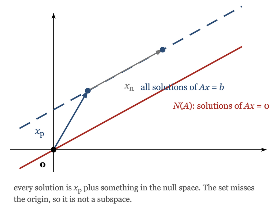
The picture shows the solution set as a line that misses the origin. Sets like that are not subspaces. To say why, we need the definitions properly.

A real vector space is a set of objects — we call them vectors — together with rules for adding two of them and for multiplying one by a real number, such that the results stay inside the set. Compactly:

One consequence follows at once, and it is the quickest test available.

Every vector space contains the zero vector. Take any \(x \in V\) and put \(\alpha = 1, \beta = -1, y = x\); then \(\alpha x + \beta y = x - x = 0\) must lie in \(V\).

Most of the sets we care about are not standalone spaces but live inside a bigger one.

Since the condition is inherited from \(V\), the only thing to check is that combinations do not escape \(W\). Two examples of failure, both instructive:

The smallest subspace of any space is \(\{0\}\), and the largest is the whole space.

We have been calling them spaces, so we had better check.

By contrast the solution set of \(Ax=b\) with \(b\neq 0\) is not a subspace, since it does not contain \(0\) (if it did, \(A0=0\) would force \(b=0\)). That is the algebra behind the figure.

Take the matrix we will use for the rest of this section,

which is \(3\times 4\) — three equations in four unknowns. Run forward elimination exactly as before. The first pivot is \(1\) in position \((1,1)\), and the multipliers are \(\ell_{21} = 2/1 = 2\) and \(\ell_{31} = -1/1 = -1\). Subtracting \(\ell_{i1}\) times row 1 from row \(i\), entry by entry,

(For row 2, column 3: \(9 - 2\times 3 = 3\). For row 3, column 3: \(3 - (-1)\times 3 = 6\). The other entries go similarly.)

Now something new happens. The natural second pivot would be in position \((2,2)\), but that entry is zero — and so is everything below it in column 2. In Chapter 1 this was the fatal case for a square matrix. Here it is not fatal at all: we simply move right, and look for a pivot in column 3. There is one, the \(3\) in position \((2,3)\). Using it, with multiplier \(\ell_{32} = 6/3 = 2\),

(Row 3, column 4: \(6 - 2\times 3 = 0\).) The last row has vanished entirely. The result \(U\) is called an echelon matrix.

Our example has pivots in columns 1 and 3, so \(r=2\). Everything from Chapter 1 survives: the row operations were still multiplications by unit lower triangular matrices, so with

we again have \(A = LU\), now with \(L\) of size \(3\times 3\) and \(U\) of size \(3\times 4\). If row exchanges are needed it becomes \(PA=LU\), as before. The multipliers land in \(L\) in place for exactly the reason proved in Chapter 1.

We can go two steps further, and it pays to do so. Divide each row by its pivot, then use each pivot to clear the entries above it as well as below. On our \(U\): divide row 2 by 3 to get \((0,0,1,1)\), and then row 1 becomes \(\text{row}_1 - 3\times\text{row}_2 = (1,3,3-3,2-3) = (1,3,0,-1)\). So

This is the reduced row echelon form (RREF): all pivots are 1, and each pivot is the only nonzero entry in its column. Unlike \(U\), which depends on the elimination path, \(R\) is uniquely determined by \(A\) — a fact we shall use but not prove.

The step from \(U\) to \(R\) is again a multiplication by an invertible matrix (this time an upper triangular one, since we were subtracting later rows from earlier ones). That matters, and here is why.

Claim 2.1. If \(M\) is invertible then \(N(MA) = N(A)\). In particular \(A\), \(U\) and \(R\) all have the same null space.

So solve \(Rx=0\) instead. Reading the two nonzero rows of \(R\),

Because each pivot column has zeros everywhere except at the pivot, each equation involves exactly one pivot variable. Split the unknowns accordingly:

The name is the recipe. The free variables may be given any values whatsoever, and the equations then determine the pivot variables: \(x_1 = -3x_2 + x_4\) and \(x_3 = -x_4\). Writing the general solution out in full,

The two vectors obtained by setting one free variable to 1 and the rest to 0 are called the special solutions. Every null space vector is a combination of them, so they span \(N(A)\). Here \(N(A)\) is a two-dimensional subspace of \(\mathbb{R}^4\) — and once again, it is not \(\mathbb{R}^2\), it is a two-dimensional flat object inside \(\mathbb{R}^4\).

These two vectors can be read the way we read the null vector of \(B\) earlier, as statements about the columns of \(A\). Writing the columns as \(v_1,v_2,v_3,v_4\), the first special solution \((-3,1,0,0)\) says \(-3v_1 + v_2 = 0\), and the second \((1,0,-1,1)\) says \(v_1 - v_3 + v_4 = 0\). That is,

Check them against \(A\): \(3v_1 = 3(1,2,-1) = (3,6,-3) = v_2\), and \(v_3 - v_1 = (3,9,3) - (1,2,-1) = (2,7,4) = v_4\). So the two free columns are combinations of the two pivot columns, and the null space records exactly which combinations. We will use this in a moment to pick out a basis for the column space.

The bookkeeping generalizes immediately. Let \(A\) be \(m\times n\) with rank \(r\).

One consequence is immediate and useful.

This also discharges a promissory note from Chapter 1. There, in proving that \(Ax=0 \Rightarrow x=0\) forces elimination to produce \(n\) pivots, we said "the corresponding unknown is free; set it to 1 and solve upwards", and deferred the bookkeeping to this chapter. The special-solution construction above is that bookkeeping: a column without a pivot gives a free variable, and setting it to 1 produces an explicit nonzero vector in the null space.

The last row of \(U\) is entirely zero, so the last equation of \(Ux=c\) reads \(0 = c_3\). There is no \(x\) on the left at all. So the system is solvable if and only if

This is the solvability condition. In general there are \(m-r\) of them, one for each zero row of \(U\), and they are conditions on \(b\) alone.

Compare this with what the column picture said: \(Ax=b\) is solvable exactly when \(b\in C(A)\). Both must be right, so they must be saying the same thing. And they are: \(5b_1 - 2b_2 + b_3 = 0\) is \(b^Ty = 0\) with \(y = (5,-2,1)\), which by the row picture of Chapter 1 describes a plane through the origin with normal \(y\). That plane is \(C(A)\). Check the columns of \(A\) against it: for column 1, \(5(1) - 2(2) + 1(-1) = 5-4-1 = 0\); for column 3, \(5(3) - 2(9) + 1(3) = 15-18+3 = 0\). Both lie in the plane, as they should. We will return to this vector \(y\); it has a name.

Take a right hand side that passes the test, say \(b = (1,5,5)\): indeed \(5(1) - 2(5) + 5 = 0\). Then \(c = (1,\, 5-2(1),\, 0) = (1,3,0)\), and \(Ux=c\) reads

To get one solution, set the free variables to zero: \(x_2 = x_4 = 0\). The second equation gives \(3x_3 = 3\), so \(x_3 = 1\). The first gives \(x_1 + 3(0) + 3(1) + 2(0) = 1\), so \(x_1 = -2\). Hence

and you should check directly that \(Ax_p = (1,5,5)\). Combining with the null space computed earlier, the complete solution is

One run of elimination produced both halves at once: setting the free variables to zero gave \(x_p\), and setting the right hand side to zero gave the null space. Note again that this set of solutions is not a subspace — the shift by \(x_p\) pushes it off the origin.

Everything about \(Ax=b\) is contained in the three numbers \(r\), \(m\), \(n\), and in the position of the pivots.

Two small cases fix the idea. If \(v_1\) and \(v_2\) are parallel, say \(v_1 = \alpha v_2\), then \(1\cdot v_1 + (-\alpha)v_2 = 0\) with a nonzero coefficient, so they are dependent. If three vectors lie in a common plane, one of them is a combination of the other two, say \(v_3 = \alpha v_1 + \beta v_2\), and then \(\alpha v_1 + \beta v_2 + (-1)v_3 = 0\) is a dependence relation. In each case the relation records the redundancy.

Now assemble the vectors as the columns of a matrix \(A\). Then \(c_1v_1 + \cdots + c_nv_n\) is precisely \(Ac\), so the definition reads: the columns of \(A\) are independent exactly when \(Ac = 0\) forces \(c=0\). In other words,

Combining this with the counting result of the previous section gives a fact that is used constantly.

Claim 2.2. Any \(n\) vectors in \(\mathbb{R}^m\) with \(n > m\) are linearly dependent.

So you cannot have three independent vectors in a plane, or five in \(\mathbb{R}^4\). Independence puts a ceiling on how many vectors you can have.

The opposite requirement is that there be enough vectors.

Spanning puts a floor on how many vectors you need. The columns of \(A\) span \(C(A)\) by definition, and the special solutions span \(N(A)\) by construction. Note that a spanning set need not give unique coefficients: in \(\mathbb{R}^3\) the four vectors \((1,0,0)\), \((0,1,0)\), \((0,0,1)\), \((1,1,1)\) certainly span, but there are infinitely many ways to write a given \(v\) using all four.

A basis is what you get when the ceiling and the floor meet.

The point of insisting on both is that the representation then becomes unique.

Claim 2.3. If \(\{v_1,\ldots,v_k\}\) is a basis for \(V\), every \(v\in V\) has exactly one expression \(v = \sum_i c_iv_i\).

These unique coefficients are the coordinates of \(v\) in the basis, and they are what let us represent an abstract vector as a concrete column of numbers. A basis is far from unique — \(\mathbb{R}^3\) has infinitely many — but once you fix one, the coordinates are pinned down.

A caution using our running example. From \(U = \begin{bmatrix} 1 & 3 & 3 & 2 \\ 0 & 0 & 3 & 3 \\ 0 & 0 & 0 & 0\end{bmatrix}\):

Different bases of the same space can look completely different. What they cannot do is differ in size.

Theorem 2.4. Any two bases of a vector space contain the same number of vectors. That number is called the dimension of the space.

Two consequences follow, and we shall use both.

Corollary 2.5. Let \(V\) have dimension \(k\). Then (i) any \(k\) independent vectors in \(V\) already form a basis of \(V\), and (ii) a subspace of \(\mathbb{R}^m\) whose dimension is \(m\) is the whole of \(\mathbb{R}^m\).

With that, "two-dimensional subspace of \(\mathbb{R}^4\)" finally means something precise. It also closes the loose end from Chapter 1 — why a single equation \(a^Tx = d\) in \(\mathbb{R}^n\) leaves an \((n-1)\)-dimensional set. For \(a\neq 0\) the homogeneous equation \(a^Tx=0\) is \(Ax=0\) for the \(1\times n\) matrix \(A = a^T\), which has one pivot, so \(r=1\) and the null space has dimension \(n-1\). For \(d\neq 0\) the solution set is that null space shifted by one particular solution, which does not change its dimension.

Before computing dimensions, we must be careful about which of these can be read off \(U\) or \(R\) and which cannot.

Claim 2.6. Elimination leaves the row space and the null space unchanged, but it need not preserve the column space.

This is why the recipe for a basis of \(C(A)\) says: find the pivot columns using \(R\), but then take those columns from \(A\), not from \(R\).

Theorem 2.7. For any \(A\) with \(r\) pivots, \(\dim C(A) = \dim C(A^T) = r\), and \(\dim N(A) = n - r\).

The equality \(\dim C(A) = \dim C(A^T)\) deserves a second look. The column space lives in \(\mathbb{R}^m\) and the row space in \(\mathbb{R}^n\); they may share nothing beyond the zero vector, and for a \(3\times 4\) matrix they do not even sit in the same space. Yet they always have the same dimension. That common value is the rank, and this is the reason the word "rank" needs no qualifier.

The relation \(\dim C(A) + \dim N(A) = r + (n-r) = n\) is the rank—​nullity statement: the column count of \(A\) splits into the part that survives and the part that is destroyed. The dimension of the null space is called the nullity of \(A\), and \(N(A)\) is also called the kernel.

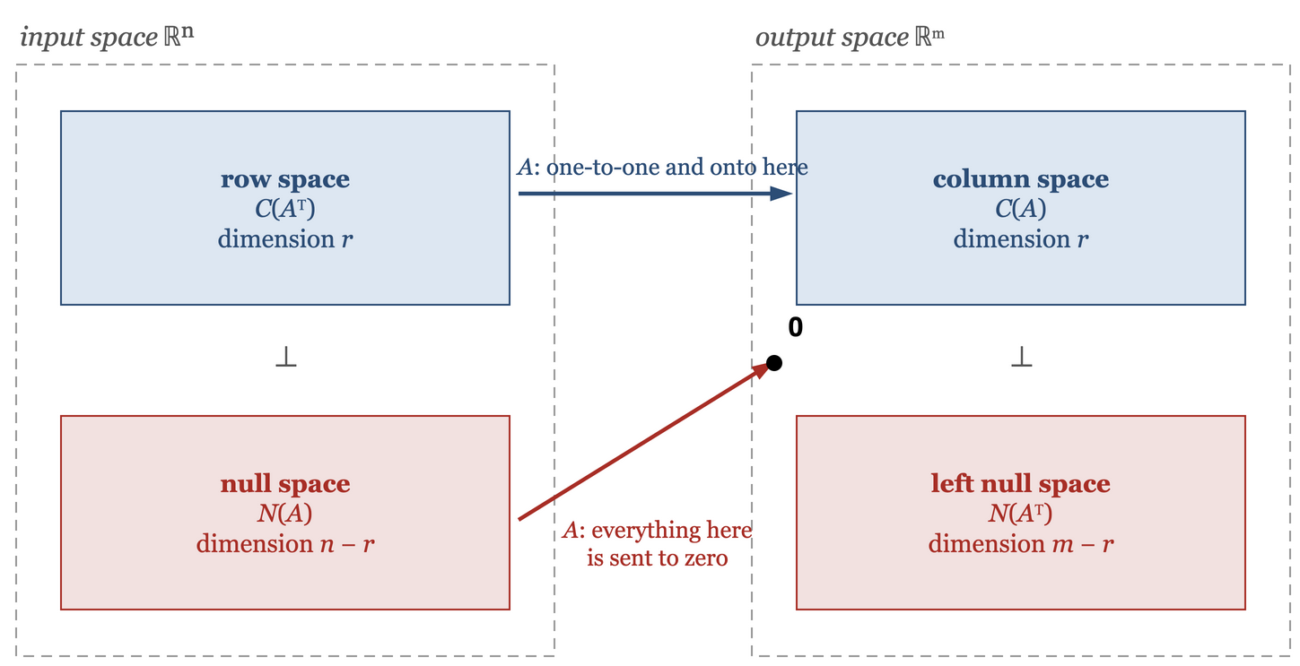
For our running example, \(m=3\), \(n=4\), \(r=2\), so the dimensions are \(2, 2, 4-2=2\) and \(3-2=1\). The left null space is one-dimensional, and its basis vector has already appeared.

A smaller case can be done completely. All four spaces are then lines, and the whole picture fits on one page. Take

whose second row is \(3\) times the first and whose second column is half the first, so \(r=1\). With \(m=n=2\), all four dimensions are \(1\). Taking each in turn:

Now look at the two right angles, which we prove in general below. In \(\mathbb{R}^2\) the row space and null space meet at one: \((2,1)\cdot(1,-2) = 2 - 2 = 0\). In the output copy of \(\mathbb{R}^2\) the column space and left null space do the same: \((1,3)\cdot(3,-1) = 3 - 3 = 0\). Four lines, two perpendicular pairs, one in each space.

The vertical splitting in the figure is not just for tidiness.

Claim 2.8. Every vector in the row space is perpendicular to every vector in the null space. Every vector in the column space is perpendicular to every vector in the left null space.

The dimensions fit this perfectly: in \(\mathbb{R}^n\) the row space has dimension \(r\) and the null space \(n-r\), adding to \(n\); in \(\mathbb{R}^m\) the column space has dimension \(r\) and the left null space \(m-r\), adding to \(m\). Each space is split into two perpendicular pieces. The chapter on orthogonality makes this precise with the term orthogonal complement and shows that the splitting is complete — that every vector in \(\mathbb{R}^n\) breaks into a row space part plus a null space part in exactly one way. For now, perpendicularity is enough.

We can now close the loop on the solvability condition \(5b_1 - 2b_2 + b_3 = 0\), and identify the vector \(y=(5,-2,1)\).

Theorem 2.9. \(Ax=b\) is solvable if and only if \(y^Tb = 0\) for every \(y \in N(A^T)\). The number of independent solvability conditions is \(m-r\), which is \(\dim N(A^T)\).

For the running example, \(m-r = 1\), so there is one condition and the left null space is one-dimensional. Its basis vector is \(y = (5,-2,1)\), and you can verify \(y^TA = 0\) directly: for column 1, \(5(1) - 2(2) + 1(-1) = 0\); for column 2, \(5(3) - 2(6) + 1(-3) = 15-12-3 = 0\); for column 3, \(5(3) - 2(9) + 1(3) = 0\); for column 4, \(5(2) - 2(7) + 1(4) = 10-14+4 = 0\).

So the mysterious combination that appeared in the last row of the elimination was never mysterious. It is a basis vector of the left null space, and "\(b\) must be perpendicular to it" is the same statement as "\(b\) must lie in the column space".

If \(r=m\) then \(\dim C(A) = m\), so \(C(A)\) is all of \(\mathbb{R}^m\) and \(Ax=b\) is solvable for every \(b\). Equivalently, there are \(m-r=0\) solvability conditions. This is the existence property. If moreover \(m<n\), there are \(n-m>0\) free variables, so the solution is never unique.

Theorem 2.10. If \(A\) is \(m\times n\) with full row rank, then \(AA^T\) is invertible and \(C = A^T(AA^T)^{-1}\) satisfies \(AC = I_m\). Such a \(C\) is called a right inverse.

The right inverse is not unique when \(m<n\); the formula above is one particular choice. A smaller example makes this concrete: for \(A = \begin{bmatrix} 4 & 0 & 0 \\ 0 & 5 & 0\end{bmatrix}\), any \(C\) whose first two rows are \((1/4,0)\) and \((0,1/5)\) works, and the third row is completely free. Setting that free row to zero recovers exactly the formula.

If \(r=n\) then there are \(n-r=0\) free variables, so \(N(A) = \{0\}\) and \(Ax=b\) has at most one solution. It may still have none, if \(b\notin C(A)\). This is the uniqueness property.

Theorem 2.11. If \(A\) is \(m\times n\) with full column rank, then \(A^TA\) is invertible and \(B = (A^TA)^{-1}A^T\) satisfies \(BA = I_n\). Such a \(B\) is a left inverse.

Putting the two together: full row rank buys existence, full column rank buys uniqueness, and a square invertible matrix has both — which is Theorem 1.9 recovered as the special case \(r=m=n\).

The expression \(x = (A^TA)^{-1}A^Tb\) should be remembered, but it must not be over-read.

Both one-sided inverses are examples of what is called a pseudo-inverse, written \(A^{+}\). The general construction waits for the singular value decomposition.

Everything so far has treated \(A\) as a table of numbers to be reduced. There is a second way to look at it. When \(A\) multiplies \(x\), it takes the vector \(x\in\mathbb{R}^n\) and produces a new vector \(Ax\in\mathbb{R}^m\). This happens at every point of \(\mathbb{R}^n\) at once: the whole space is transformed.

The four subspaces describe what that transformation does. Everything in the null space is sent to zero. What is left is the row space, and on it nothing is lost.

Claim 2.12. \(A\) carries the row space one-to-one and onto the column space.

This is what the four-subspace picture is recording. The chapter on orthogonality completes it, by showing that every \(x\in\mathbb{R}^n\) splits in exactly one way into a row space part plus a null space part, so that the two halves of the figure account for all of \(\mathbb{R}^n\).

Four small examples in the plane show the range of behaviour. In each, a matrix acts on every point \((x,y)\) at once.

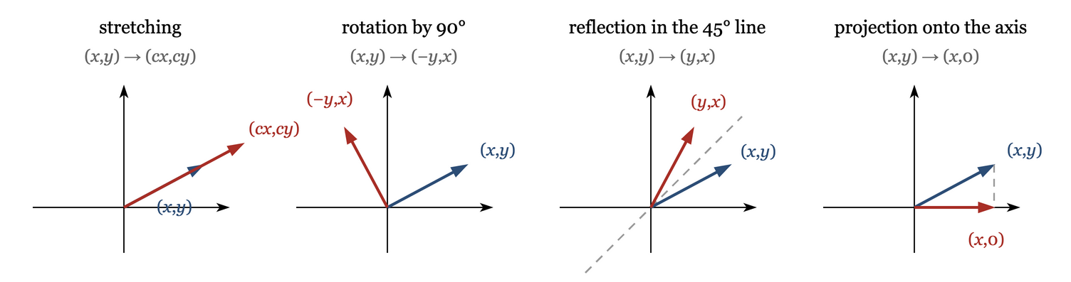
The first, \(cI\), stretches every vector by the same factor \(c\); the whole plane expands or contracts. The second sends \((x,y)\) to \((-y,x)\), a rotation of everything through \(90^\circ\). The third swaps the coordinates, which is reflection in the \(45^\circ\) line \(y=x\) — note that it is also a permutation matrix, so simple algebraically that the geometry is easy to miss. The fourth sends \((x,y)\) to \((x,0)\), projecting the plane onto the horizontal axis; here the column space is that axis and the null space is the vertical axis, which is crushed to the origin. The same four ideas lift to three dimensions: stretch the earth, spin it, reflect it in the plane of the equator, or flatten it onto that plane.

Just as instructive is the list of things no matrix can do to a space.

Rule 2 contains rule 1, by taking \(c=0\). We have in fact been using rule 3 all along: when the reflection above acts on \((4,0)\), we may split it as \((2,2) + (2,-2)\), reflect each piece separately to get \((2,2)\) and \((-2,2)\), and add, giving \((0,4)\). Splitting, transforming and adding is legitimate precisely because of rule 3.

Those rules are important enough to be made the definition, and rules 2 and 3 collapse into one requirement.

Every matrix gives a linear transformation, immediately. The interesting question runs the other way: does every linear transformation give a matrix? For maps between \(\mathbb{R}^n\) and \(\mathbb{R}^m\) the answer is yes, and the proof tells you how to build the matrix.

Claim 2.13. Let \(T:\mathbb{R}^n\rightarrow\mathbb{R}^m\) be linear. Then there is a matrix \(A\) with \(T(x) = Ax\) for all \(x\), namely the matrix whose \(j\)-th column is \(T(e_j)\).

So a linear transformation is completely determined by what it does to a basis. Fix the images of \(n\) basis vectors and every other value follows. Every construction below is an application of this.

Nothing in the definition of a linear transformation mentions columns of numbers; it needs only addition and scaling. So it applies verbatim to the polynomial space \(P_n\), whose vectors are \(p(t) = a_0 + a_1t + \cdots + a_nt^n\). Its natural basis is the list of \(n+1\) polynomials

These span \(P_n\) by the definition of a polynomial, and they are independent: a combination of them that vanishes for every \(t\) is a polynomial of degree at most \(n\) with infinitely many roots, and only the zero polynomial does that, so all the coefficients are zero. Hence \(\dim P_n = n+1\).

Differentiation. The map \(T = d/dt\) sends \(P_n\) to \(P_{n-1}\):

It is linear, since the derivative of a combination is that combination of the derivatives. Its null space is the set of constants \(p = a_0\), which is one-dimensional; its column space is all of \(P_{n-1}\), of dimension \(n\). And indeed \(1 + n = n+1\), the dimension of \(P_n\) — rank—​nullity again, in a space that has nothing to do with columns of numbers.

Integration. The map \(p \mapsto \int_0^t p(\tau)\,d\tau\) sends \(P_n\) to \(P_{n+1}\):

It is linear, and its null space is \(\{0\}\) — only the zero polynomial integrates to zero.

Once a basis is fixed, each vector gets a column of coordinates, and we need a notation for it. Write

For \(P_n\) with the natural basis, \([p]_B\) is just \((a_0,a_1,\ldots,a_n)\). The bracket is extra notation, but it prevents a confusion that comes up often.

For this reason we will name the bases rather than the basis vectors, and always say which basis a coordinate column is written in.

To turn such a transformation into a matrix, use the fact just established. The recipe needs two bases.

Differentiation as a matrix. Take \(V = P_4\) with basis \(B = \{1,t,t^2,t^3,t^4\}\) and \(W = P_3\) with basis \(C = \{1,t,t^2,t^3\}\). The action on each vector of \(B\) is \(T(1) = 0\), \(T(t) = 1\), \(T(t^2) = 2t\), \(T(t^3) = 3t^2\), \(T(t^4) = 4t^3\). Reading each result in the output basis \(C\) gives the columns:

Test it on \(p = t + 2t^2 - 4t^3 + t^4\), whose coordinate column in \(B\) is \([p]_B = (0,1,2,-4,1)\) — five entries, because \(B\) has five vectors. Multiplying, the first entry is \(0(0)+1(1)+0(2)+0(-4)+0(1) = 1\), the second is \(2(2) = 4\), the third is \(3(-4) = -12\), the fourth is \(4(1) = 4\). So \(A_{\text{diff}}\,p = (1,4,-12,4)\), i.e. \(1 + 4t - 12t^2 + 4t^3\), which is what differentiating \(p\) by hand gives.

Integration as a matrix. Take \(V = P_3\) with basis \(C = \{1,t,t^2,t^3\}\) and \(W=P_4\) with basis \(B = \{1,t,t^2,t^3,t^4\}\) — the same two lists as before, now swapped between input and output. Note that \(C\) is a basis of \(P_3\) and \(B\) of \(P_4\), so the columns of the matrix below have five entries where the previous one had four. Now \(T(1) = t\), \(T(t) = t^2/2\), \(T(t^2) = t^3/3\), \(T(t^3) = t^4/4\), so

The first row is zero because the constant term of an integral starting at \(0\) is always zero — the output basis vector \(y_1 = 1\) is never used.

If \(U \xrightarrow{B} V \xrightarrow{A} W\) are two linear transformations, then doing one after the other is again linear, and its matrix is the product: \(w = Av = A(Bu) = (AB)u\). Matrix multiplication was defined so that this works.

A pleasing example: \(A_{\text{diff}}\) is \(4\times 5\) and \(A_{\text{int}}\) is \(5\times 4\), so \(A_{\text{diff}}A_{\text{int}}\) is \(4\times 4\), and multiplying them out gives \(I_4\). Integrating and then differentiating returns the polynomial you started with, which is the fundamental theorem of calculus in matrix form. The other order does not give the identity: \(A_{\text{int}}A_{\text{diff}}\) is \(5\times 5\) and cannot be \(I_5\), because differentiation has a null space (the constants) and anything with a null space is not invertible. Concretely, differentiating \(p = 3\) and then integrating returns \(0\), not \(3\) — the constant is lost.

So \(A_{\text{diff}}\) is a left inverse of \(A_{\text{int}}\) but not a right inverse, which is precisely the rectangular situation of the previous section: \(A_{\text{int}}\) has full column rank (nullity zero) and therefore has a left inverse, but not a right one.

These are the standard transformations of the plane. In each case the method is the same: find the images of the two basis vectors \(x_1 = (1,0)\) and \(x_2 = (0,1)\), and use them as the columns.

Rotation by \(\theta\). The vector \((1,0)\) rotates to \((\cos\theta, \sin\theta)\). The vector \((0,1)\) rotates to \((-\sin\theta, \cos\theta)\). Hence

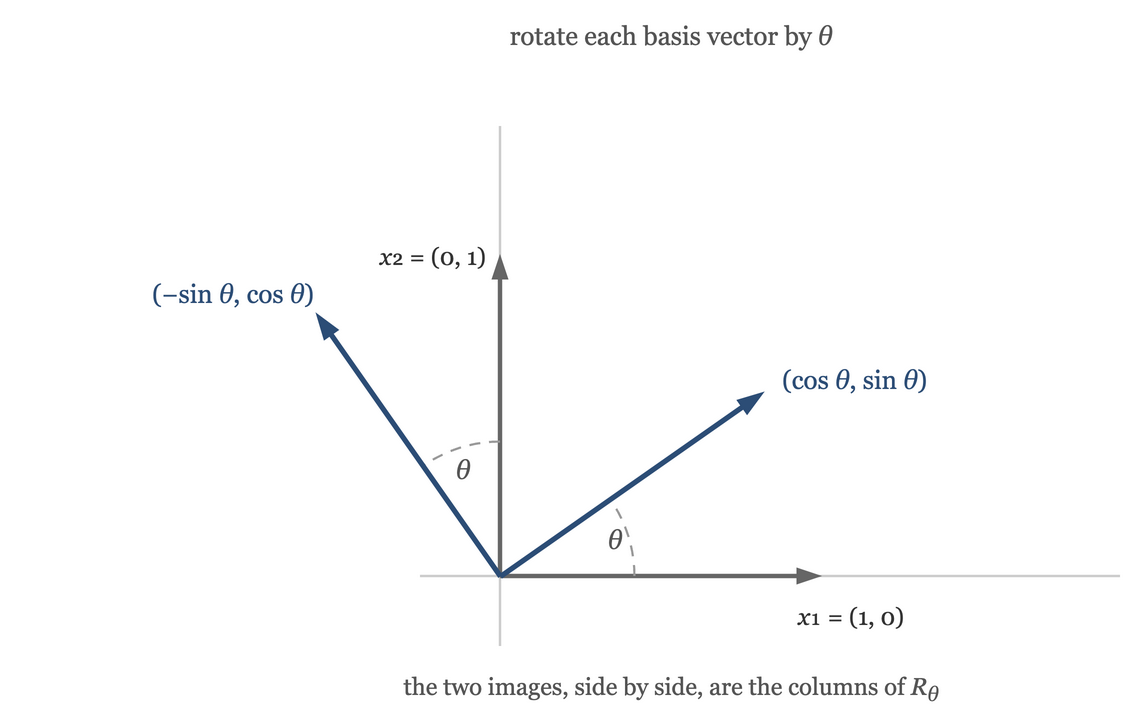
Rotating by \(\theta\) and then by \(\phi\) should be the same as rotating by \(\theta+\phi\), and the matrices agree: multiplying \(R_\phi R_\theta\), the \((1,1)\) entry is \(\cos\phi\cos\theta - \sin\phi\sin\theta = \cos(\theta+\phi)\), and the other three entries work out the same way, giving \(R_\phi R_\theta = R_{\theta+\phi}\). The addition formulae of trigonometry drop out of matrix multiplication.

Projection onto a line through the origin at angle \(\theta\). Project \((1,0)\): it has length 1 and makes angle \(\theta\) with the line, so its shadow on the line has length \(\cos\theta\), and that shadow as a vector is \(\cos\theta\,(\cos\theta,\sin\theta) = (\cos^2\theta, \sin\theta\cos\theta)\). Project \((0,1)\): it makes angle \(90^\circ - \theta\) with the line, so its shadow has length \(\sin\theta\), giving \(\sin\theta\,(\cos\theta,\sin\theta) = (\sin\theta\cos\theta, \sin^2\theta)\). So

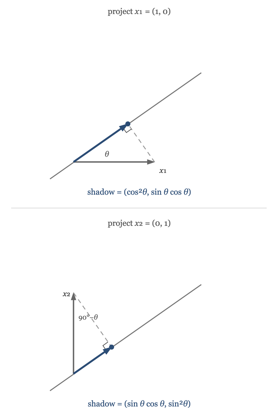
Three things follow at once. Its null space is the line through the origin perpendicular to the projection line, since everything on that perpendicular has zero shadow — so \(P\) is not invertible. Its column space is the projection line itself. And projecting a second time changes nothing, because a point already on the line is its own shadow: \(P^2 = P\). (Verify the algebra: the \((1,1)\) entry of \(P^2\) is \(\cos^2\theta\cos^2\theta + \sin\theta\cos\theta\sin\theta\cos\theta = \cos^2\theta(\cos^2\theta+\sin^2\theta) = \cos^2\theta\).)

Reflection in the same line. If \(b = Pa\) is the shadow of \(a\), then the reflected point \(a'\) is obtained by travelling from \(a\) to \(b\) and then the same distance again, so \(a' = a + 2(b - a) = 2b - a\). Hence

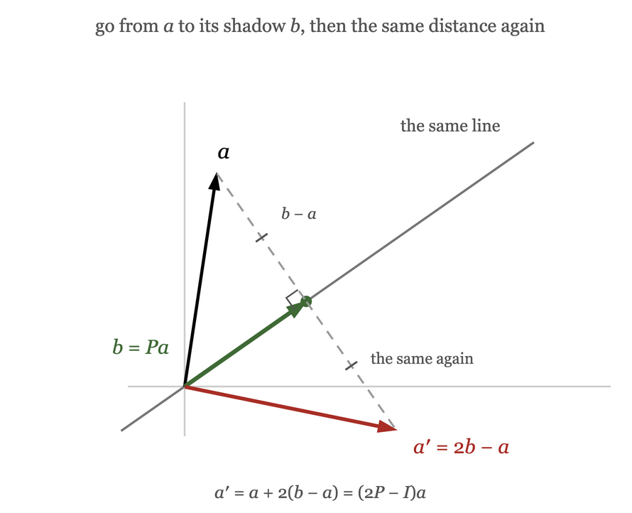
Reflecting twice must return you to where you started, and it does: using \(P^2 = P\),

One last point, and it is the one that opens the next chapters. The matrix representing a transformation is not a property of the transformation alone. It depends on the bases you chose.

Take the projection \(P\) above. In the standard basis it is the rather unpleasant matrix of sines and cosines. But suppose we choose a new basis adapted to the problem: \(v_1\) along the projection line, and \(v_2\) perpendicular to it. Then the transformation is trivial to describe — \(v_1\) is unchanged and \(v_2\) is sent to zero — so its matrix in that basis is

Similarly the reflection \(H\) keeps \(v_1\) and flips \(v_2\), so in the same basis it is \(\mathrm{diag}(1,-1)\). The same transformations, and much simpler matrices; all that changed was the point of view.

That raises an obvious question: given a matrix, is there a basis in which it becomes as simple as possible — ideally diagonal? The vectors that such a basis would have to consist of are those that \(A\) merely scales, \(Ax = \lambda x\). These are the eigenvectors, and finding them is the subject of the eigenvalue problem, the second of the two equations this course is built around.