Having established the first-order necessary (KKT) conditions, we now revisit them through a worked example and then develop the theory of duality, which lets us attack a constrained (primal) problem through an associated (dual) problem.
A motivating example
Start with the objective \(f(x) = \frac{2}{5}(x_1^2 + x_2^2)\) and solve the constrained problem
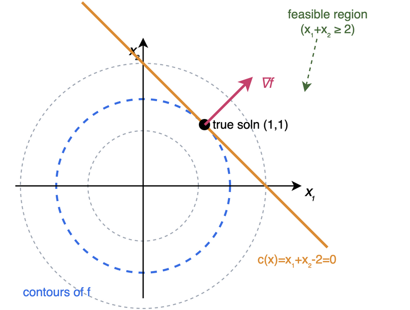
The Lagrangian is \(\mathcal{L}(x,\lambda) = f(x) - \lambda c(x)\). As per the KKT conditions, at an optimal \(x^*\) we require \(\nabla_x \mathcal{L}(x^*,\lambda^*) = 0\) with \(\lambda^* \ge 0\) and the complementarity condition \(\lambda^* c(x^*) = 0\). The stationarity condition reads
Let us test two candidate points:
-
What if \(x = \frac{5}{4}\begin{bmatrix} 1 \\ 1\end{bmatrix}\)? Then \(\lambda = 1\), but \(c(x) = \frac{5}{4}+\frac{5}{4}-2 = \frac12 \ne 0\), so \(\lambda c(x) \ne 0\) — complementarity fails.
-
What if \(x^* = \begin{bmatrix} 1 \\ 1\end{bmatrix}\)? Then \(\lambda = 0.8\), and \(c(x) = 0\) (so \(\lambda c(x) = 0\)). All KKT conditions are satisfied at \((1,1)\). Since \(\nabla c(x) = \begin{bmatrix}1 & 1\end{bmatrix}^T \ne 0\), LICQ holds, so the optimal multiplier is unique.
Solving the same problem via the dual
Let us solve P1 differently, in two steps.
Step 1 — Define the Lagrangian dual function:
For a fixed (not-yet-optimal) \(\lambda\), the inner minimum occurs where \(\nabla_x \mathcal{L}(x,\lambda) = 0\):
Substituting back,
Step 2 — Find \(\lambda \ge 0\) that maximizes \(q(\lambda)\):
the same answer as before. What did we just do?
Primal and dual problems
The dual problem is called the Lagrangian dual problem. In general, when equality constraints are also present, the constraint above becomes \(\lambda_i \ge 0\;\forall i \in \mathcal{I}\) (only the inequality multipliers are sign-constrained).
Two remarks:
-
It is not guaranteed to always work; it works for a class of problems.
-
When it works, it leads to a simpler optimization problem.
Proofs come later; we develop the geometry now.
Geometric view of duality
Our usual (primal) problem is in \(x = (x_1, x_2)\) space. Let’s map it to another space given by \((y=c(x), z=f(x))\) via
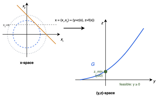
Every point \((x_1,x_2)\) is mapped into a region \(G\) in \((y,z)\) coordinates, and feasibility is now just \(y \ge 0\). To see the shape of \(G\), fix \(x_2 = a\); then \(y = x_1 + a - 2\) and
so each horizontal line \(x_2 = a\) maps to a parabola; for \(a = 0\), \(z = \frac{2}{5}(y+2)^2\). The geometry is now clear.
-
What is the primal problem? \(\underset{}{\text{min}}\; z\) while \(y \ge 0\). The marked point \(z_{\text{min}}\) on the \(z\)-axis is the solution.
-
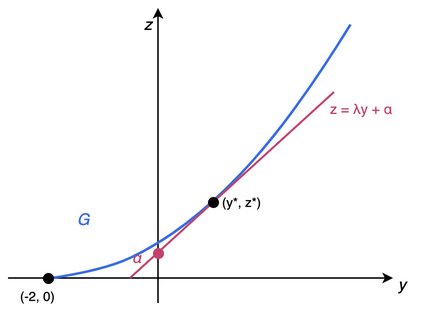
What is the dual problem? Visualize \(\mathcal{L}(x,\lambda) = f(x) - \lambda c(x) = \alpha\) (say), i.e. \(\alpha = z - \lambda y\), or \(z = \lambda y + \alpha\). What is this geometrically? A line of slope \(\lambda\) and intercept \(\alpha\) on the \(z\) axis.
Let’s solve this in two steps:
Step 1 (dual function). For fixed \(\lambda\),
In words: what is the minimum possible value of the intercept \(\alpha\), while keeping at least one point \((y,z) \in G\)?
But why is \(q(\lambda)\) finite at all — why can’t we slide the line down forever and drive \(\alpha \to -\infty\)? Because \(G\) is not the whole plane; it is bounded below. For a fixed \(y\) (i.e. fixed \(x_1+x_2=y+2\)), \(z=f\) is smallest when \(x_1 = x_2 = \frac{y+2}{2}\), giving \(z = \frac{1}{5}(y+2)^2\) — the \(a=0\) slice drawn above is just one curve sitting above this envelope. Thus
the region on and above this parabola; in particular \(z \ge 0\), touching \(z=0\) only at the vertex \((-2,0)\). A slope-\(\lambda\) line slid downwards therefore jams against this parabolic floor — push it past the point of tangency and the whole line drops below \(G\), meeting nothing. So the smallest reachable intercept is finite, and that value is exactly \(q(\lambda)\). (The weaker fact \(z\ge 0\) alone would not pin it down: a tilted line could run off along \(z=0\) as \(y\to\infty\); it is the parabola’s quadratic growth outpacing \(\lambda y\) that supplies the floor.)
Step 2 (dual optimum). Finally,
while maintaining the definition of \(q\) (which needs legitimate feasible \((y,z)\) points). That is, we maximize the intercept by varying \(\lambda\).
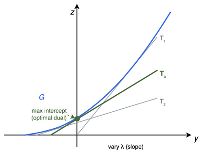
In this example the optimal primal value \(z^*\) equals the optimal dual value — they are equal, so there is no gap: this is strong duality.
Properties of the dual
Recall \(q(\lambda) = \underset{x}{\text{min}}\; \mathcal{L}(x,\lambda)\). It can happen that for some \(\lambda\), \(q(\lambda) \to -\infty\). We therefore define the domain of \(q\) as
There are two important results, true for any \(f, c\):
-
\(q\) is concave.
-
\(\mathcal{D}\) is convex.
Implication: solving the dual problem is a convex optimization problem — regardless of the primal problem.
Proof of (1) — concavity. Consider \(\lambda_1, \lambda_2\) and \(\alpha \in [0,1]\). Since \(\mathcal{L}(x,\lambda) = f(x) - \lambda c(x)\) is affine in \(\lambda\),
Taking \(\underset{x}{\text{min}}\) of both sides and using \(\underset{x}{\text{min}}(a+b) \ge \underset{x}{\text{min}}\,a + \underset{x}{\text{min}}\,b\) (e.g. \(a = x, b = -x\)),
Proof of (2) — convexity of \(\mathcal{D}\). In words, convexity of \(\mathcal{D}\) means: if \(\lambda_1 \in \mathcal{D}\) and \(\lambda_2 \in \mathcal{D}\), then \((1-\alpha)\lambda_1 + \alpha\lambda_2 \in \mathcal{D}\) too. Given \(\lambda_1, \lambda_2 \in \mathcal{D}\), we have \(q(\lambda_1) > -\infty\) and \(q(\lambda_2) > -\infty\). By the concavity of \(q\) just proved,
Thus a convex combination of \(\lambda_1, \lambda_2\) is also in \(\mathcal{D}\), i.e. \(\mathcal{D}\) is a convex set. To summarize: the primal problem can be anything, but the dual problem is always concave.
Weak duality
For the primal \(\underset{x}{\text{min}}\; f(x)\) s.t. \(c(x) \ge 0\): for any feasible \(\bar{x}\) and any \(\bar\lambda \ge 0\), the following holds:
Important corollary. Define the optimal primal and dual values
Then \(q^\circ \le f^\circ\): the optimum of the dual problem never exceeds the optimum of the primal. Consequently:
-
If \(q^\circ < f^\circ\), then \(f^\circ - q^\circ > 0\) is called a duality gap.
-
If \(q^\circ = f^\circ\), we have strong duality.
-
For convex optimization problems, the duality gap is always \(0\) under a constraint qualification (e.g. LICQ).
Worked example using duality
Consider
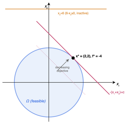
Primal. The objective level sets are \(-(x_1+x_2) = c \implies x_2 = -x_1 - c\); we want the minimum value of \(c\). Geometrically the solution is \(x^* = (2,2)\) with \(f^\circ = -4\). The problem is convex, so we expect the dual problem to give the same solution.
Dual.
-
The Lagrangian (with \(\lambda_i \ge 0\)):
\[\begin{align*} \mathcal{L}(x,\lambda) &= f(x) - \sum_i \lambda_i c_i(x) = -(x_1 + x_2) - \lambda_1(8 - x_1^2 - x_2^2) - \lambda_2(6 - x_2) \\ &= -\big[ -\lambda_1 x_1^2 - \lambda_1 x_2^2 + x_1 + x_2(1 - \lambda_2) + 8\lambda_1 + 6\lambda_2 \big], \end{align*}\]which is clearly a convex function of \(x\) (for \(\lambda_1 > 0\)).
-
\(q(\lambda) = \underset{x}{\text{min}}\; \mathcal{L}(x,\lambda)\); by the observation above this minimization makes sense. Setting \(\nabla_x \mathcal{L} = 0\):
\[\begin{equation*} \nabla_x \mathcal{L} = \begin{bmatrix} 2\lambda_1 x_1 - 1 \\ 2\lambda_1 x_2 - 1 + \lambda_2 \end{bmatrix} = 0 \implies x_1^\circ = \frac{1}{2\lambda_1}, \quad x_2^\circ = \frac{1 - \lambda_2}{2\lambda_1}. \end{equation*}\]Substituting back,
\[\begin{align*} q(\lambda) &= \lambda_1(x_1^{\circ 2} + x_2^{\circ 2}) - x_1^\circ + (\lambda_2 - 1)x_2^\circ - 8\lambda_1 - 6\lambda_2 \\ &= \frac{1 + (1-\lambda_2)^2}{4\lambda_1} - \frac{1}{2\lambda_1} - \frac{(1-\lambda_2)^2}{2\lambda_1} - 8\lambda_1 - 6\lambda_2 = -\frac{1 + (1-\lambda_2)^2}{4\lambda_1} - 8\lambda_1 - 6\lambda_2. \end{align*}\] -
The dual problem is \(\underset{\lambda \ge 0}{\text{max}}\; q(\lambda)\). (One can verify concavity explicitly via \(\nabla q, \nabla^2 q\), or invoke the proof of the previous section.) Writing the maximization as a minimization of the negative,
\[\begin{equation*} \underset{\lambda \ge 0}{\text{max}}\; q(\lambda) = -\underset{\lambda \ge 0}{\text{min}}\; \left[ \frac{1 + (1-\lambda_2)^2}{4\lambda_1} + 8\lambda_1 + 6\lambda_2 \right], \qquad \lambda_1 \ge 0,\; \lambda_2 \ge 0. \end{equation*}\]
This inner minimization is itself a constrained problem, but it can be solved analytically. Introduce multipliers \(\mu_1, \mu_2\) for \(\lambda_1 \ge 0, \lambda_2 \ge 0\):
with the KKT conditions \(\mu_1, \mu_2 \ge 0\) and \(\mu_1 \lambda_1 = 0,\; \mu_2 \lambda_2 = 0\). Now \(\lambda_1 = 0\) is not a solution (as \(W\) blows up), so \(\mu_1 = 0\). Then \(\nabla_\lambda W = 0\) gives
Two cases:
-
\(\mu_2 > 0 \implies \lambda_2 = 0\). Then \(\frac{-2}{4\lambda_1^2} + 8 = 0 \implies \lambda_1 = \frac14\), and \(\frac{2(-1)}{4\lambda_1} + 6 - \mu_2 = -2 + 6 - \mu_2 = 0 \implies \mu_2 = 4 \ge 0\) — feasible.
-
\(\mu_2 = 0 \implies \frac{\lambda_2 - 1}{2\lambda_1} = -6 \implies \lambda_2 = 1 - 12\lambda_1\). Then \(1 + (1-\lambda_2)^2 = 32\lambda_1^2 \implies 1 + 144\lambda_1^2 = 32\lambda_1^2 \implies 112\lambda_1^2 + 1 = 0\) — not possible.
So the only KKT point is \(\begin{bmatrix} \lambda_1 \\ \lambda_2 \end{bmatrix} = \begin{bmatrix} 1/4 \\ 0 \end{bmatrix}\), which leads to
This is the same as \(f^\circ = -4\), so we have strong duality. The recovered primal point is